YOLO,你想知道的都在这
YOLO
- 推荐CSDN学院课程: YOLOv3目标检测:原理与源码解析
- YOLO 的前世今生
-
- YOLOv1
-
- YOlOv1的损失函数
- YOLOv2
- YOLOv3
-
- 正负样本是什么?
- YOLOv3 全部都是卷积层,舍弃了全连接层,那么如何转换的呢:
-
- FCN
- 卷积stride某种程度上等价于滑动窗口
- 物体标签框的中心坐标,落在哪个格子里,哪个就负责预测这个物体!
- Anchor预测
-
- 为啥用anchor?
-
- 如何一个网格预测多个物体?
- Objectness Score
- Class Confidences
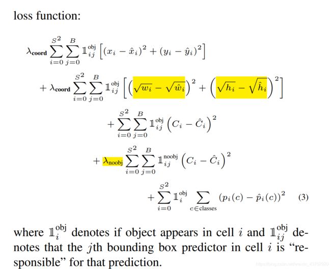
- YOLOv3的损失函数
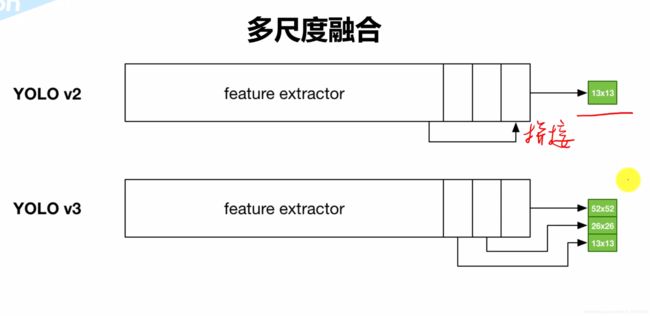
- 跨尺度预测
- 权重初始化,weight initialization
- C实现解析
-
- 过程
- cfg文件
- Pytorch 实现
-
- 如何计算IOU?
- train.py
- xyxy <==> xywh 坐标转换
- 图片变换后的框坐标
- mAP
- 未完待续。。。
英文原文
推荐CSDN学院课程: YOLOv3目标检测:原理与源码解析
YOLO 的前世今生
YOLOv1
- 最早的YOLO,一个grid cell 预测B个bounding boxes 和一组 概率,每个bouding box又预测了四个坐标值和一个confidence。因此最终有 S × S × ( B ∗ 5 + C ) S\times S\times (B*5+C) S×S×(B∗5+C).重点在,一个格子
只会预测一组conditional class probabilities. - 最早的YOLO并不是FCN而是有
2层全连接层 - 最早的YOLO,anchor boxes没有应用。
- 回归的损失乘以0.5权重(5 × \times × 回归框损失),1 × \times × 分类损失,1 × \times × 有物体的confidence损失,0.5 × \times × 没有物体时候的confidence损失,1 × \times × 类别的条件概率损失.
YOlOv1的损失函数
- 只用了传统的 dropout(也要缩放矫正) 和数据增强,记得矫正GT框防止过拟合
- 数据增强包括,随机剪裁,旋转,HSV变换shift等
- 激活用 Leaky ReLu
- YOLOv1在
定位和Recall上表现差! - yolo 224 × 224 224\times224 224×224 训练,用224*2输入,想通过分辨率大的图片提升获取更清晰的特征。
YOLOv2
-
加入了BN层,加速收敛。减少权重初始化的依赖。防止过拟合舍弃dropout。
-
不同于上面的8, v2用416*416输入大小,为了让feature map 有个中心网格!比如
13*13
-
不同与上面的1,这次,每个anchor box都要预测一组条件类别概率!因此也就是 S × S × B ∗ ( 5 + C ) S\times S\times B*(5+C) S×S×B∗(5+C)
-
抛弃全连接层,使用全卷积层FCN
-
使用了5个Anchor Boxes机制,mAP降低了0.3%,但是recall上升了7%.

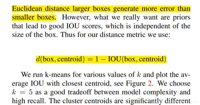
- 有创造性的是用 K-means算法自动得到anchor box, 不用手动hand-pick. 纵轴为平均IOU
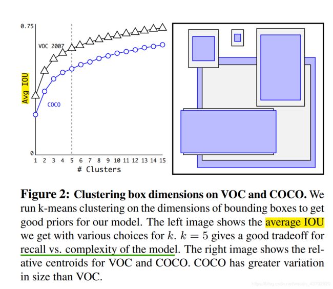
- K-means的距离选择不是欧氏距离,而是1-IOU。因为大的box, 明显会产生较大的误差。例如: ( 100 − 95 ) 2 = 25 , ( 1 − 0.95 ) 2 = 0.0 5 2 (100-95)^2 =25, (1-0.95)^2=0.05^2 (100−95)2=25,(1−0.95)2=0.052
这里是引用自传送门
- 多尺度训练!每10batches改变输入的大小,由于网络downsample的factor是
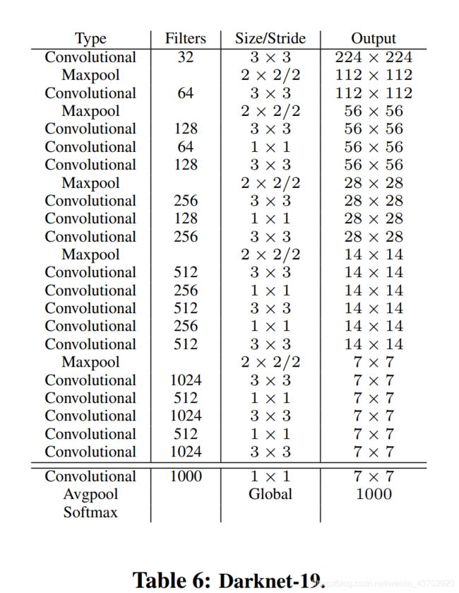
32,为了方便,就用32的倍数,范围为(320,608)=(10,19)*32 - 大部分目标检测网络基于VGG16。虽然准确,但是运算量大: 30.69 billions。YOLO基于GoogleNet架构。准确率低了2%,运算量只有 8.52 billions。YOLO2最终模型基础为Darkent-19(19层卷积层)。
- 然后YOLO900论文中有意思的是,Jointly Training!综合检测数据集(框回归,分类),分类数据集(只有类别标签)训练,对应不同的损失部分。分类数据集只考虑分类的损失。
YOLOv3
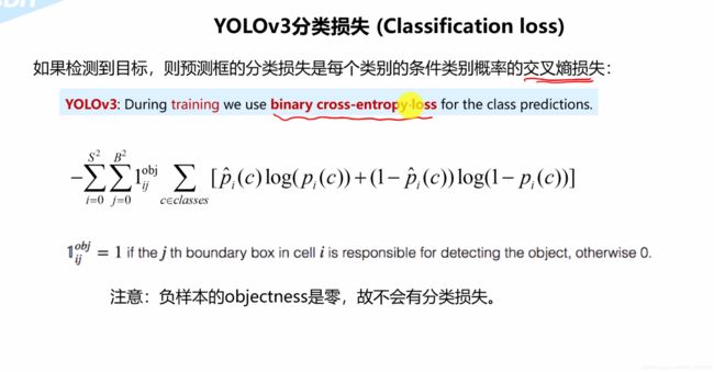
- 分类用多标签的独立逻辑斯特回归,损失函数为二分类交叉熵函数 Binary CrossEntropy
- 这次用三个尺度一共
9个anchor boxes!
- 新的特征提取网络Darkent-53!
这里没有maxpooling池化层,因为只需要进行卷积就可以实现下采样了,而且不会丢失空间的信息。
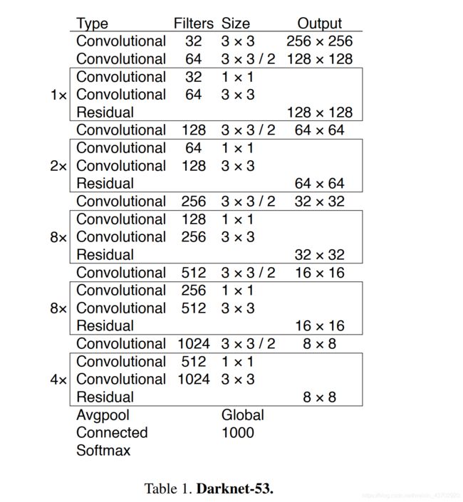
- 还是比较优秀的。计算量比ResNet大一些。

- 成果,虽然RetinaNet各方面领先,但是训练时长要3.8倍于Yolov3。
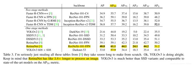
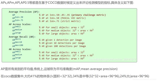
一些指标参数介绍,引用自传送门
正负样本是什么?
YOLOv3 全部都是卷积层,舍弃了全连接层,那么如何转换的呢:
FCN
如下图,上面 是带有全连接层的神经网络,我们需要的预测的是4个类别的概率。
同理我们也可以用 卷积 神经网络 构成一样的结构。
只要通过一个和前一层被卷积张量一样大小的kernel size,就行了。
下图是 5 × 5 × 16 5 \times\ 5 \times16 5× 5×16输入张量和400 个 5 × 5 × 16 5 \times 5 \times16 5×5×16卷积体卷积后得到 1 × 1 × 400 1\times1\times400 1×1×400张量,也就是和上图的400神经元的全连接层等价。
卷积stride某种程度上等价于滑动窗口
-
以往的滑动窗口目标检测,就是选择一个框大小,然后在原图上从左到右从上到下,一次次滑动,然后得到一次次预测。
-
每一次滑动就有一个预测向量(车,人,树…)。我们可以通过预测向量中最大的概率对应的框作为预测框。
滑动框的缺点:
- 这种方法问题在于你的滑动框定死了!
- 第二个问题: 框之间重复计算了
重复计算,诶? 因此自然而然想到用卷积来操作,因为本身就和卷积操作相似了。
- 举例
下图第三行,等价于用第一行的 14 × 14 × 3 14\times14\times3 14×14×3窗口,滑动得到的预测图。
换句话说,某输入张量矩阵经过多层卷积层后,得到一个多维的输出张量矩阵。这个输出矩阵,可以看做是对每一个输入张量矩阵中的相同滑动框大小,不同位置的预测值!
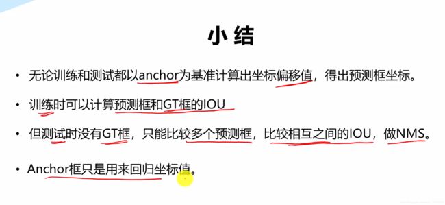
物体标签框的中心坐标,落在哪个格子里,哪个就负责预测这个物体!
-
作为FCN,YOLOv3本是可以改变输入大小的
无视图片大小。但是,实际上,由于各种问题,我们可能希望保持不变的输入大小,而这些问题只会在实现算法时浮出水面。 -
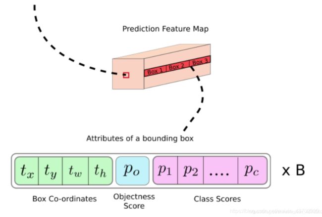
Feature map通过最后一层 1 × 1 1\times1 1×1 卷积后得到 Prediction Map(预测图)
Prediction Map中每一个Cell预测了固定数目的回归框。 -
Depth-wise, we have ( B x (4+1 + C) ) entries in the feature map:
深度方向上,最后的feature map 有 ( B x (5 +C) ) 个元素,每个BOX有5+C个预测值
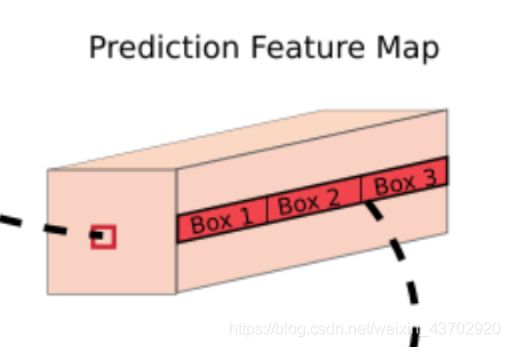
( o b j e c t n e n e s S c o r e + C l a s s e s P r o b a b i l i t y + t x + t y + t w + t h ) ∗ B o u d i n g B o x e s ( objectnenesScore+ClassesProbability+ t_x +t_ y +t_ w +t_h )* BoudingBoxes (objectnenesScore+ClassesProbability+tx+ty+tw+th)∗BoudingBoxes
o b j e c t n e n e s S c o r e = c o n f i d e n c e = P ( o b j e c t ) ∗ I O U P r e d T r u t h objectnenes \space Score = confidence =P(object)*IOU_{Pred}^{Truth} objectnenes Score=confidence=P(object)∗IOUPredTruth
举例如下:
下图大小为13 x 13
标签框的中心 落在(7,7),因此这个cell负责预测狗,这个尺度上(13*13尺度)可以预测3个Bouding box。
实际上,yolo有三个尺度图的预测,下图只是一个13*13大小的如同格子一样的预测图,每个预测图的每个格子预测了不同大小的三个框。
| 检测大尺度(13,13) | 中尺度 (26,26) | 检测小尺度(52,52) |
|---|---|---|
| 小一点的三个固定框10,13, 16,30, 33,23, | 中等的三个固定框 30,61, 62,45, 59,119, | 大的三个固定框 116,90, 156,198, 373,326 |
总结一下!
我们找到了哪个格子负责预测我们的物体,但是框的大小怎么预测??
Anchor预测
为啥用anchor?
传送门
借用Andrew的动图:
如何一个网格预测多个物体?
蓝色花括号代表着Anchors,如果里面有目标,则希望对应的部分,objectiveness score=1
预测边界框的宽度和高度可能是有意义的,但在实践中,这会导致在训练过程中出现不稳定的梯度。相反,大多数现代object detector预测log_space transformation ,或者简单地偏移到预定义的默认包围框(称为锚)。
Then, these transforms are applied to the anchor boxes to obtain the prediction.
YOLO v3 has three anchors, which result in prediction of three bounding boxes per cell.
负责检测狗的框将是和标签框具有最大IOU的Anchor框。
请再看图:
这里的
t x , t y , t w , t h t_x ,t_y, t_w, t_h tx,ty,tw,th
这四个坐标并不是最终(绘制)的坐标,而是相对中心的偏离scale坐标!
bx, by, bw, bh are the x,y center co-ordinates, width and height of our prediction. tx, ty, tw, th is what the network outputs. cx and cy are the top-left co-ordinates of the grid. pw and ph are anchors dimensions for the box.
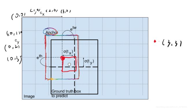
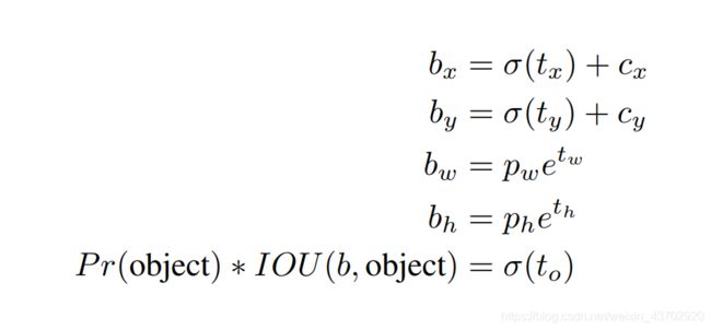
bx, by, bw, bh are the x,y center co-ordinates, width and height of our prediction.
注意:
这个 b w , b h b_w,b_h bw,bh是相对于feature map大小的=归一化比例=,比如你的 b w , b h b_w,b_h bw,bh 为 ( 0.3 , 0.8 ) (0.3,0.8) (0.3,0.8),那么你的实际预测框的大小为 ( 13 × 0.3 , 13 × 0.8 ) (13\times0.3,13\times0.8) (13×0.3,13×0.8)
- 那么为什么要用sigmoid函数?
使得预测的cell不会偏离中心cell!
the output is passed through a sigmoid function, which squashes the output in a range from 0 to 1, effectively keeping the center in the grid which is predicting.
Objectness Score
学习过后,中心的红框子的概率基本为1,周围的各自概率接近1,边缘的格子为0
Class Confidences
在yolov3之前使用softmax预测类别概率,但是导致的问题就是,如果目标属于某一类,它就不能属于另一类。这在Woman和Person这种分类情况下就不使用。因此就是用sigmoid来预测。
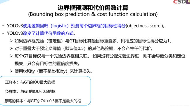
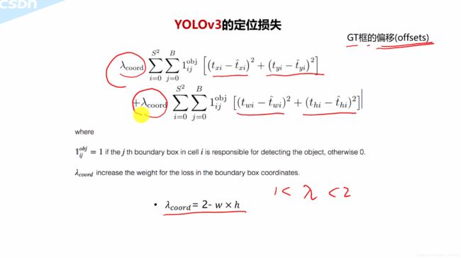
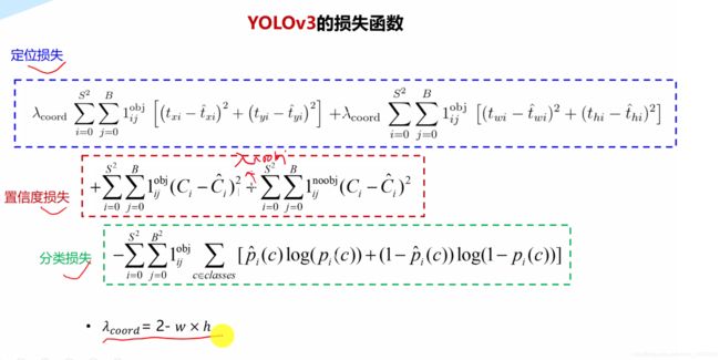
YOLOv3的损失函数
YOLOv1是softmax后进行平方差损失
跨尺度预测
三个预测尺度:
412 × 412 412\times412 412×412大小的图片输入
| 检测大尺度(13,13) | 中尺度 (26,26) | 检测小尺度(52,52) |
|---|---|---|
| 32 | 16 | 8 |
跨尺度说明产生了很多预测框(10647个框),怎么筛选到最终的1个框
3 × ( 13 × 13 ) + 3 × ( 26 × 26 ) + 3 × ( 52 × 52 ) = 10647 3\times(13\times13)+3\times(26\times26)+3\times(52\times52)=10647 3×(13×13)+3×(26×26)+3×(52×52)=10647
- 通过上面的objectness score,框具有低于阈值的score直接排除忽视掉。
- NMS非极大值抑制
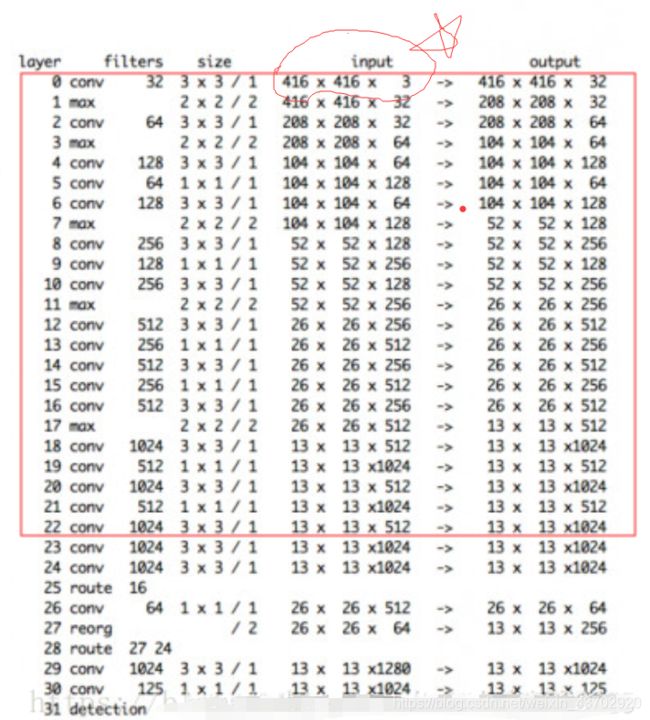
网络结构图,concatenate目的是把前面的位置信息和后面的语义信息融合
权重初始化,weight initialization
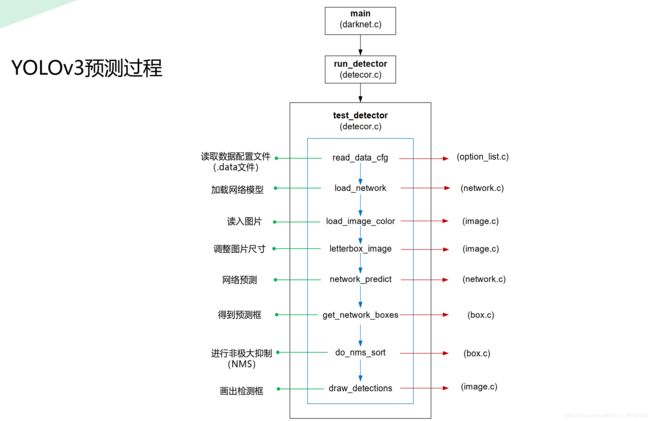
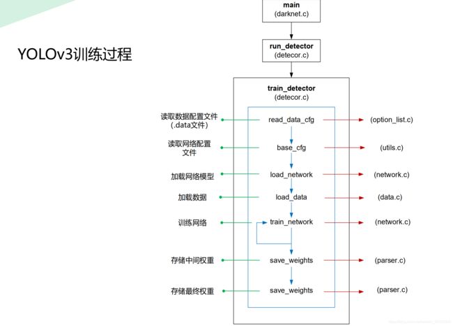
C实现解析
过程
预测和训练
cfg文件
Pytorch 实现
如何计算IOU?
def bbox_iou(box1, box2):
    """
    Returns the IoU of two bounding boxes
    """
    #Get the coordinates of bounding boxes
    b1_x1, b1_y1, b1_x2, b1_y2 = box1[:,0], box1[:,1], box1[:,2], box1[:,3]
    b2_x1, b2_y1, b2_x2, b2_y2 = box2[:,0], box2[:,1], box2[:,2], box2[:,3]

    #get the corrdinates of the intersection rectangle
    inter_rect_x1 =  torch.max(b1_x1, b2_x1)
    inter_rect_y1 =  torch.max(b1_y1, b2_y1)
    inter_rect_x2 =  torch.min(b1_x2, b2_x2)
    inter_rect_y2 =  torch.min(b1_y2, b2_y2)

    #Intersection area
    inter_area = torch.clamp(inter_rect_x2 - inter_rect_x1 + 1, min=0) * torch.clamp(inter_rect_y2 - inter_rect_y1 + 1, min=0)

    #Union Area
    b1_area = (b1_x2 - b1_x1 + 1)*(b1_y2 - b1_y1 + 1)
    b2_area = (b2_x2 - b2_x1 + 1)*(b2_y2 - b2_y1 + 1)

    iou = inter_area / (b1_area + b2_area - inter_area)

    return iou
layer filters size input output
0 conv 32 3 x 3 / 1 416 x 416 x 3 -> 416 x 416 x 32 0.299 BF
1 conv 64 3 x 3 / 2 416 x 416 x 32 -> 208 x 208 x 64 1.595 BF
2 conv 32 1 x 1 / 1 208 x 208 x 64 -> 208 x 208 x 32 0.177 BF
3 conv 64 3 x 3 / 1 208 x 208 x 32 -> 208 x 208 x 64 1.595 BF
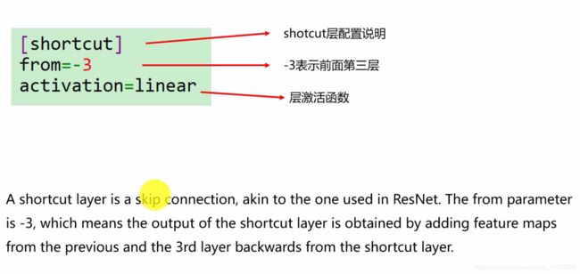
4 Shortcut Layer: 1
5 conv 128 3 x 3 / 2 208 x 208 x 64 -> 104 x 104 x 128 1.595 BF
6 conv 64 1 x 1 / 1 104 x 104 x 128 -> 104 x 104 x 64 0.177 BF
7 conv 128 3 x 3 / 1 104 x 104 x 64 -> 104 x 104 x 128 1.595 BF
8 Shortcut Layer: 5
9 conv 64 1 x 1 / 1 104 x 104 x 128 -> 104 x 104 x 64 0.177 BF
10 conv 128 3 x 3 / 1 104 x 104 x 64 -> 104 x 104 x 128 1.595 BF
11 Shortcut Layer: 8
12 conv 256 3 x 3 / 2 104 x 104 x 128 -> 52 x 52 x 256 1.595 BF
13 conv 128 1 x 1 / 1 52 x 52 x 256 -> 52 x 52 x 128 0.177 BF
14 conv 256 3 x 3 / 1 52 x 52 x 128 -> 52 x 52 x 256 1.595 BF
15 Shortcut Layer: 12
16 conv 128 1 x 1 / 1 52 x 52 x 256 -> 52 x 52 x 128 0.177 BF
17 conv 256 3 x 3 / 1 52 x 52 x 128 -> 52 x 52 x 256 1.595 BF
18 Shortcut Layer: 15
19 conv 128 1 x 1 / 1 52 x 52 x 256 -> 52 x 52 x 128 0.177 BF
20 conv 256 3 x 3 / 1 52 x 52 x 128 -> 52 x 52 x 256 1.595 BF
21 Shortcut Layer: 18
22 conv 128 1 x 1 / 1 52 x 52 x 256 -> 52 x 52 x 128 0.177 BF
23 conv 256 3 x 3 / 1 52 x 52 x 128 -> 52 x 52 x 256 1.595 BF
24 Shortcut Layer: 21
25 conv 128 1 x 1 / 1 52 x 52 x 256 -> 52 x 52 x 128 0.177 BF
26 conv 256 3 x 3 / 1 52 x 52 x 128 -> 52 x 52 x 256 1.595 BF
27 Shortcut Layer: 24
28 conv 128 1 x 1 / 1 52 x 52 x 256 -> 52 x 52 x 128 0.177 BF
29 conv 256 3 x 3 / 1 52 x 52 x 128 -> 52 x 52 x 256 1.595 BF
30 Shortcut Layer: 27
31 conv 128 1 x 1 / 1 52 x 52 x 256 -> 52 x 52 x 128 0.177 BF
32 conv 256 3 x 3 / 1 52 x 52 x 128 -> 52 x 52 x 256 1.595 BF
33 Shortcut Layer: 30
34 conv 128 1 x 1 / 1 52 x 52 x 256 -> 52 x 52 x 128 0.177 BF
35 conv 256 3 x 3 / 1 52 x 52 x 128 -> 52 x 52 x 256 1.595 BF
36 Shortcut Layer: 33
37 conv 512 3 x 3 / 2 52 x 52 x 256 -> 26 x 26 x 512 1.595 BF
38 conv 256 1 x 1 / 1 26 x 26 x 512 -> 26 x 26 x 256 0.177 BF
39 conv 512 3 x 3 / 1 26 x 26 x 256 -> 26 x 26 x 512 1.595 BF
40 Shortcut Layer: 37
41 conv 256 1 x 1 / 1 26 x 26 x 512 -> 26 x 26 x 256 0.177 BF
42 conv 512 3 x 3 / 1 26 x 26 x 256 -> 26 x 26 x 512 1.595 BF
43 Shortcut Layer: 40
44 conv 256 1 x 1 / 1 26 x 26 x 512 -> 26 x 26 x 256 0.177 BF
45 conv 512 3 x 3 / 1 26 x 26 x 256 -> 26 x 26 x 512 1.595 BF
46 Shortcut Layer: 43
47 conv 256 1 x 1 / 1 26 x 26 x 512 -> 26 x 26 x 256 0.177 BF
48 conv 512 3 x 3 / 1 26 x 26 x 256 -> 26 x 26 x 512 1.595 BF
49 Shortcut Layer: 46
50 conv 256 1 x 1 / 1 26 x 26 x 512 -> 26 x 26 x 256 0.177 BF
51 conv 512 3 x 3 / 1 26 x 26 x 256 -> 26 x 26 x 512 1.595 BF
52 Shortcut Layer: 49
53 conv 256 1 x 1 / 1 26 x 26 x 512 -> 26 x 26 x 256 0.177 BF
54 conv 512 3 x 3 / 1 26 x 26 x 256 -> 26 x 26 x 512 1.595 BF
55 Shortcut Layer: 52
56 conv 256 1 x 1 / 1 26 x 26 x 512 -> 26 x 26 x 256 0.177 BF
57 conv 512 3 x 3 / 1 26 x 26 x 256 -> 26 x 26 x 512 1.595 BF
58 Shortcut Layer: 55
59 conv 256 1 x 1 / 1 26 x 26 x 512 -> 26 x 26 x 256 0.177 BF
60 conv 512 3 x 3 / 1 26 x 26 x 256 -> 26 x 26 x 512 1.595 BF
61 Shortcut Layer: 58
62 conv 1024 3 x 3 / 2 26 x 26 x 512 -> 13 x 13 x1024 1.595 BF
63 conv 512 1 x 1 / 1 13 x 13 x1024 -> 13 x 13 x 512 0.177 BF
64 conv 1024 3 x 3 / 1 13 x 13 x 512 -> 13 x 13 x1024 1.595 BF
65 Shortcut Layer: 62
66 conv 512 1 x 1 / 1 13 x 13 x1024 -> 13 x 13 x 512 0.177 BF
67 conv 1024 3 x 3 / 1 13 x 13 x 512 -> 13 x 13 x1024 1.595 BF
68 Shortcut Layer: 65
69 conv 512 1 x 1 / 1 13 x 13 x1024 -> 13 x 13 x 512 0.177 BF
70 conv 1024 3 x 3 / 1 13 x 13 x 512 -> 13 x 13 x1024 1.595 BF
71 Shortcut Layer: 68
72 conv 512 1 x 1 / 1 13 x 13 x1024 -> 13 x 13 x 512 0.177 BF
73 conv 1024 3 x 3 / 1 13 x 13 x 512 -> 13 x 13 x1024 1.595 BF
74 Shortcut Layer: 71
75 conv 512 1 x 1 / 1 13 x 13 x1024 -> 13 x 13 x 512 0.177 BF
76 conv 1024 3 x 3 / 1 13 x 13 x 512 -> 13 x 13 x1024 1.595 BF
77 conv 512 1 x 1 / 1 13 x 13 x1024 -> 13 x 13 x 512 0.177 BF
78 conv 1024 3 x 3 / 1 13 x 13 x 512 -> 13 x 13 x1024 1.595 BF
79 conv 512 1 x 1 / 1 13 x 13 x1024 -> 13 x 13 x 512 0.177 BF
80 conv 1024 3 x 3 / 1 13 x 13 x 512 -> 13 x 13 x1024 1.595 BF
81 conv 18 1 x 1 / 1 13 x 13 x1024 -> 13 x 13 x 18 0.006 BF
82 yolo
83 route 79
84 conv 256 1 x 1 / 1 13 x 13 x 512 -> 13 x 13 x 256 0.044 BF
85 upsample 2x 13 x 13 x 256 -> 26 x 26 x 256
86 route 85 61
87 conv 256 1 x 1 / 1 26 x 26 x 768 -> 26 x 26 x 256 0.266 BF
88 conv 512 3 x 3 / 1 26 x 26 x 256 -> 26 x 26 x 512 1.595 BF
89 conv 256 1 x 1 / 1 26 x 26 x 512 -> 26 x 26 x 256 0.177 BF
90 conv 512 3 x 3 / 1 26 x 26 x 256 -> 26 x 26 x 512 1.595 BF
91 conv 256 1 x 1 / 1 26 x 26 x 512 -> 26 x 26 x 256 0.177 BF
92 conv 512 3 x 3 / 1 26 x 26 x 256 -> 26 x 26 x 512 1.595 BF
93 conv 18 1 x 1 / 1 26 x 26 x 512 -> 26 x 26 x 18 0.012 BF
94 yolo
95 route 91
96 conv 128 1 x 1 / 1 26 x 26 x 256 -> 26 x 26 x 128 0.044 BF
97 upsample 2x 26 x 26 x 128 -> 52 x 52 x 128
98 route 97 36
99 conv 128 1 x 1 / 1 52 x 52 x 384 -> 52 x 52 x 128 0.266 BF
100 conv 256 3 x 3 / 1 52 x 52 x 128 -> 52 x 52 x 256 1.595 BF
101 conv 128 1 x 1 / 1 52 x 52 x 256 -> 52 x 52 x 128 0.177 BF
102 conv 256 3 x 3 / 1 52 x 52 x 128 -> 52 x 52 x 256 1.595 BF
103 conv 128 1 x 1 / 1 52 x 52 x 256 -> 52 x 52 x 128 0.177 BF
104 conv 256 3 x 3 / 1 52 x 52 x 128 -> 52 x 52 x 256 1.595 BF
105 conv 18 1 x 1 / 1 52 x 52 x 256 -> 52 x 52 x 18 0.025 BF
106 yolo
train.py
- 混合精度训练
mixed_precision = True
try:  # Mixed precision training https://github.com/NVIDIA/apex
    from apex import amp
except:
    print('Apex recommended for faster mixed precision training: https://github.com/NVIDIA/apex')
    mixed_precision = False  # not installed
xyxy <==> xywh 坐标转换
def xyxy2xywh(x):
    # Convert nx4 boxes from [x1, y1, x2, y2] to [x, y, w, h] where xy1=top-left, xy2=bottom-right
    # xy1是左上角, xy2是右下角
    y = torch.zeros_like(x) if isinstance(x, torch.Tensor) else np.zeros_like(x)
    y[:, 0] = (x[:, 0] + x[:, 2]) / 2  # x center
    y[:, 1] = (x[:, 1] + x[:, 3]) / 2  # y center
    y[:, 2] = x[:, 2] - x[:, 0]  # width
    y[:, 3] = x[:, 3] - x[:, 1]  # height
    return y

def xywh2xyxy(x):
    # Convert nx4 boxes from [x, y, w, h] to [x1, y1, x2, y2] where xy1=top-left, xy2=bottom-right
    y = torch.zeros_like(x) if isinstance(x, torch.Tensor) else np.zeros_like(x)
    y[:, 0] = x[:, 0] - x[:, 2] / 2  # top left x
    y[:, 1] = x[:, 1] - x[:, 3] / 2  # top left y
    y[:, 2] = x[:, 0] + x[:, 2] / 2  # bottom right x
    y[:, 3] = x[:, 1] + x[:, 3] / 2  # bottom right y
    return y
图片变换后的框坐标
- clip_boards 用来使得坐标在矩形内
- 图中的坐标变换
def clip_coords(boxes, img_shape):
    # Clip bounding xyxy bounding boxes to image shape (height, width)
    boxes[:, 0].clamp_(0, img_shape[1])  # x1
    boxes[:, 1].clamp_(0, img_shape[0])  # y1
    boxes[:, 2].clamp_(0, img_shape[1])  # x2
    boxes[:, 3].clamp_(0, img_shape[0])  # y2

def scale_coords(img1_shape, coords, img0_shape, ratio_pad=None):
    # Rescale coords (xyxy) from img1_shape to img0_shape
    if ratio_pad is None:  # calculate from img0_shape
        gain = max(img1_shape) / max(img0_shape)  # gain  = old / new
        pad = (img1_shape[1] - img0_shape[1] * gain) / 2, (img1_shape[0] - img0_shape[0] * gain) / 2  # wh padding
    else:
        gain = ratio_pad[0][0]
        pad = ratio_pad[1]

    coords[:, [0, 2]] -= pad[0]  # x padding
    coords[:, [1, 3]] -= pad[1]  # y padding
    coords[:, :4] /= gain
    clip_coords(coords, img0_shape)
    return coords
mAP
- 已知 tp, confidence, pred_cls, target_cls
- np.argsort() 返回对数组排序(递增)的索引
- np.unique()函数去除其中重复的元素,并排序后返回