18_2Reinforcement Learning_\r_end=““_Deep Q-Learning_Double DQN_Dueling DQN_TF-Agents
cp18_Reinforcement Learning for Markov Decision Making in Env_Bellman_Q-learning_Q-Value Iteration : https://blog.csdn.net/Linli522362242/article/details/117889535
18_Reinforcement Learning_CartPole_reduce_mean_Q-Value Iteration_Q-learning_DQN_get_weights_replay :
https://blog.csdn.net/Linli522362242/article/details/117673730
https://arxiv.org/pdf/1509.06461.pdf
Deep Q-Learning Variants
Let’s look at a few variants of the Deep Q-Learning algorithm that can stabilize and speed up training.
Fixed Q-Value Targets
In the basic Deep Q-Learning algorithm, the model is used both to make predictions and to set its own targets. This can lead to a situation analogous to a dog chasing its own tail. This feedback loop can make the network unstable: it can diverge, oscillate, freeze, and so on. To solve this problem, in their 2013 paper the DeepMind researchers used two DQNs instead of one: the first is the online model, which learns at each step and is used to move the agent around, and the other is the target model used only to define the targets. The target model is just a clone of the online model:

import tensorflow as tf
from tensorflow import keras
import numpy as np
import gym

keras.backend.clear_session()
tf.random.set_seed(42)
np.random.seed(42)

env = gym.make("CartPole-v1")
n_outputs = 2     # == env.action_space.n

# online model, which learns at each step and is used to move the agent around
model = keras.models.Sequential([
                                  keras.layers.Dense( 32, activation="elu", input_shape=[4] ),
                                  keras.layers.Dense( 32, activation="elu" ),
                                  keras.layers.Dense( n_outputs )
                                ])

# target model used only to define the targets, it is just a clone of the online model
target = keras.models.clone_model( model ) ##### target model
target.set_weights( model.get_weights() )  #####
def sample_experiences( batch_size ):
indices = np.random.randint( len(replay_memory), size=batch_size )
batch = [ replay_memory[index] for index in indices ]
# [ [states], [actions], [rewards], [next_states], [dones] ]
states, actions, rewards, next_states, dones = [ np.array([ experience[field_index]
for experience in batch
])
for field_index in range(5)
]
return states, actions, rewards, next_states, dones
batch_size = 32
discount_rate = 0.95
optimizer = keras.optimizers.Adam( learning_rate=6e-3 ) ########
loss_fn = keras.losses.Huber() ####### Suppose you want to train a regression model, but your training set is a bit noisy( if you have a lot of outliers in the training set). Of course, you start by trying to clean up your dataset by removing or fixing the outliers, but that turns out to be insufficient; the dataset is still noisy. Which loss function should you use? The mean squared error might penalize large errors too much and cause your model to be imprecise. The mean absolute error would not penalize outliers as much, but training might take a while to converge, and the trained model might not be very precise. This is probably a good time to use the Huber loss ( OR
OR introduced in https://blog.csdn.net/Linli522362242/article/details/106433059, The Huber loss is quadratic when the error is smaller than a threshold δ (typically 1) but linear when the error is larger than δ. The linear part makes it less sensitive to outliers than the mean squared error, and the quadratic part allows it to converge faster and be more precise than the mean absolute error) instead of the good old MSE.https://blog.csdn.net/Linli522362242/article/details/107294292
Previously, we mentioned that just a few episodes later, it forgot everything it knew, and its performance dropped below 50! This is called catastrophic forgetting灾难性遗忘, and it is one of the big problems facing virtually all RL algorithms: as the agent explores the environment, it updates its policy, but what it learns in one part of the environment may break what it learned earlier in other parts of the environment. The experiences(Transitions) are quite correlated, and the learning environment keeps changing ==> this case leads ==> a lot of outliers
Then, in the training_step() function, we just need to change one line to use the target model instead of the online model when computing the Q-Values of the next states:
    if episode % 50 == 0:                     # for stabilizing training per 50 episode
      target.set_weights( model.get_weights() ) # use online model's weight to update target model's
Later in this chapter, we will use the TF-Agents library to train a DQN agent to play Breakout using these hyperparameters, but before we get there, let’s take a look at another DQN variant that managed to beat the state of the art once more.
Since the target model is updated much less often than the online model, the Q-Value targets are more stable, the feedback loop we discussed earlier is dampened[ˈdæmpənd]抑制, and its effects are less severe. This approach was one of the DeepMind researchers’ main contributions in their 2013 paper, allowing agents to learn to play Atari games from raw pixels. To stabilize training, they used a tiny learning rate of 0.00025, they updated the target model only every 10,000 steps (instead of the 50 in the previous code example), and they used a very large replay buffer of 1 million experiences. They decreased epsilon very slowly, from 1 to 0.1 in 1 million steps, and they let the algorithm run for 50 million steps.
Double DQN
In a 2015 paper,(Hado van Hasselt et al., “Deep Reinforcement Learning with Double Q-Learning,” Proceedings of the 30th AAAI Conference on Artificial Intelligence (2015): 2094–2100.) DeepMind researchers tweaked their DQN algorithm, increasing its performance and somewhat stabilizing training. They called this variant Double DQN. The update was based on the observation that the target network is prone to overestimating Q-Values. Indeed, suppose all actions are equally good: the Q-Values estimated by the target model should be identical, but since they are approximations, some may be slightly greater than others, by pure chance. The target model will always select the largest Q-Value, which will be slightly greater than the mean Q-Value, most likely overestimating the true Q-Value (a bit like counting the height of the tallest random wave when measuring the depth of a pool). To fix this, they proposed using the online model instead of the target model when selecting the best actions for the next states, and using the target model only to estimate the Q-Values for these best actions. Here is the updated training_step() function:
https://arxiv.org/pdf/1509.06461.pdf![]()
Notice that the selection of the action, in the argmax, is still due to the online model weights ![]() . This means that, as in Qlearning, we are still estimating the value of the greedy policy according to the current values, as defined by
. This means that, as in Qlearning, we are still estimating the value of the greedy policy according to the current values, as defined by ![]() . However, we use the second set of weights
. However, we use the second set of weights ![]() (from the target model)to fairly evaluate the value of current policy.
(from the target model)to fairly evaluate the value of current policy.
The update to the target network(target model) stays unchanged from DQN, and remains a periodic copy of the online network(online model). This version of Double DQN is perhaps the minimal possible change to DQN towards Double Q-learning. The goal is to get most of the benefit of Double Q-learning, while keeping the rest of the DQN algorithm intact for a fair comparison, and with minimal computational overhead.
##############
Equation 18-7. Target Q-Value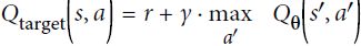
My understanding is that first target_Q_values(next_states, next_actions) is to correct the Q_values obtained by the current model, and now two DQNs are used, which can make the target model get target_Q_values(next_states, next_actions) and the estimated value obtained by the online model Q_values(states, actions) produce corresponding causal relationships (because online model (next_states, next_actions) and target model (next_states, next_actions) are corresponding, otherwise the next_actions in target_Q_values may not be the same with the acions in online model )
##############
loss_fn( target_Q_values, Q_values)
def training_step( batch_size ):

  experiences = sample_experiences( batch_size )
  states, actions, rewards, next_states, dones = experiences #(OR called transition)

  # online model, which learns at each step and is used to move the agent around
  #                                            next_states ==> online model
  next_Q_values = model.predict( next_states )           # ==> next_Q_values
  # Q_values shape: (states, actions)                    # ==> np.argmax
  best_next_actions = np.argmax( next_Q_values, axis=1 ) # ==> best_next_actions
  # e.g. actions [1, 1, 0, ...] ==>  [[0, 1], [0, 1], [1, 0],...]
  next_mask = tf.one_hot( best_next_actions, n_outputs ).numpy() # ==> next_best_actions_mask

  # next_states ==> target model ==> Q_values * next_best_actions_mask
  # ==> next_best_Q_values
  next_best_Q_values = ( target.predict( next_states )*next_mask ).sum( axis=1 )
  target_Q_values = ( rewards + (1-dones)*discount_rate * next_best_Q_values )
  target_Q_values = target_Q_values.reshape(-1,1)

  mask = tf.one_hot( actions, n_outputs )
  with tf.GradientTape() as tape:
    all_Q_values = model( states )
    Q_values = tf.reduce_sum( all_Q_values * mask,
                              axis = 1,
                              keepdims = True
                            )
    loss = tf.reduce_mean( loss_fn( target_Q_values, Q_values) )

  grads = tape.gradient( loss, model.trainable_variables )
  optimizer.apply_gradients( zip(grads, model.trainable_variables) )
https://blog.csdn.net/Linli522362242/article/details/117673730
from collections import deque

replay_memory = deque( maxlen=2000 )
def epsilon_greedy_policy( state, epsilon=0 ):
if np.random.rand() < epsilon:
# OR
# return np.random.choice(n_outputs)
# OR
# import random.randrange(2)
# random.randrange()
return np.random.randint( n_outputs )
else:
Q_values = model.predict( state[np.newaxis] )# ==>(batch_size, input_shape)
return np.argmax( Q_values[0] ) # maximum of Q_values at current state ~ action(goes to left or right)
def play_one_step( env, state, epsilon ):
action = epsilon_greedy_policy( state, epsilon )
next_state, reward, done, info = env.step( action )
replay_memory.append( (state, action, reward, next_state, done) )
return next_state, reward, done, info
env.seed(42)
np.random.seed(42)
tf.random.set_seed(42)
rewards = []
best_score = 0
for episode in range(600):
obs = env.reset()
for step in range(200):
epsilon = max( 1-episode/500, 0.01)
obs, reward, done, info = play_one_step( env, obs, epsilon )
if done:
break
rewards.append( step )
if step >= best_score:
best_weights = model.get_weights()
best_score = step
print("\rEpisode: {}, Step: {}, eps: {:.3f}".format( episode, step+1, epsilon ),
end=""
)
if episode >= 50:
training_step( batch_size )
if episode % 50 == 0: # for stabilizing training per 50 episode
target.set_weights( model.get_weights() ) # use online model's weight to update target model's
model.set_weights( best_weights ) Finally, in the training loop, we must copy the weights of the online model to the target model, at regular intervals (e.g., every 50 episodes):
![]()
import matplotlib.pyplot as plt
plt.figure( figsize=(8,4) )
plt.plot( rewards )
plt.xlabel( "Episode", fontsize=14 )
plt.ylabel( "Sum of rewards", fontsize=14 )
plt.show() 
Just a few months later, another improvement to the DQN algorithm was proposed.
Prioritized Experience Replay
Instead of sampling experiences uniformly from the replay buffer, why not sample important experiences more frequently? This idea is called importance sampling (IS) or prioritized experience replay (PER), and it was introduced in a 2015 paper(Tom Schaul et al., “Prioritized Experience Replay,” arXiv preprint arXiv:1511.05952 (2015).) by DeepMind researchers (once again!).
More specifically, experiences are considered “important” if they are likely to lead to fast learning progress. But how can we estimate this? One reasonable approach is to measure the magnitude of the TD error δ = r + γ·V(s′) – V(s). A large TD error indicates that a transition (s, r, s′) is very surprising, and thus probably worth learning from.(It could also just be that the rewards are noisy, in which case there are better methods for estimating an experience’s importance (see the paper for some examples).) When an experience is recorded in the replay buffer, its priority is set to a very large value, to ensure that it gets sampled at least once. However, once it is sampled (and every time it is sampled), the TD error δ is computed, and this experience’s priority is set to p = |δ| (plus a small constant to ensure that every experience has a nonzero probability of being sampled). The probability P of sampling an experience with priority p is proportional to ![]() 进行采样的概率 P 与
进行采样的概率 P 与 ![]() 成正比, where ζ is a hyperparameter that controls how greedy we want importance sampling to be:
成正比, where ζ is a hyperparameter that controls how greedy we want importance sampling to be:
- when ζ = 0, we just get uniform sampling, and
- when ζ = 1, we get full-blown importance sampling全面的重要性抽样.
- In the paper, the authors used ζ = 0.6, but the optimal value will depend on the task.
There’s one catch, though: since the samples will be biased toward important experiences, we must compensate for this bias during training by downweighting the experiences according to their importance, or else the model will just overfit the important experiences. To be clear, we want important experiences to be sampled more often, but this also means we must give them a lower weight during training. To do this, we define each experience’s training weight as w=![]() ,
,
- where n is the number of experiences in the replay buffer, and
- β is a hyperparameter that controls how much we want to compensate for the importance sampling bias (0 means not at all, while 1 means entirely).
- In the paper, the authors used β = 0.4 at the beginning of training and linearly increased it to β = 1 by the end of training. Again, the optimal value will depend on the task, but if you increase one, you will usually want to increase the other as well.
Now let’s look at one last important variant of the DQN algorithm.
Dueling DQN
The Dueling DQN algorithm (DDQN, not to be confused with Double DQN, although both techniques can easily be combined) was introduced in yet another 2015 paper(Ziyu Wang et al., “Dueling Network Architectures for Deep Reinforcement Learning,” arXiv preprint arXiv:
1511.06581 (2015).) by DeepMind researchers. To understand how it works, we must first note that the Q-Value of a state-action pair (s, ) can be expressed as Q(s, ) = V(s) +A(s, ), where
- V(s) is the value of state s and
- A(s, ) is the advantage of taking the action in state s, compared to all other possible actions in that state s.
- https://blog.csdn.net/Linli522362242/article/details/117889535 When the environment dynamics are known(we know the state-transition probabilities of the environment), we can easily infer the action-value function from a state-value function(one state s ~ multiple actions: state-value) by looking one step ahead to find the action that gives the maximum value
 , state, s, and action, , ==>
 ) (The difference between action-value
 and state-value
 ==>
==> is the action advantage function (“A-value”)
 ).
).
- Moreover, the value of a state(state-value) is equal to the Q-Value of the best action * for that state (since we assume the optimal policy will pick the best action), so V(s) = Q(s, *), which implies that A(s, *) = 0.
In a Dueling DQN, the model estimates both the value of the state(state-value) and the advantage of each possible action. Since the best action should have an advantage of 0, the model subtracts the maximum predicted advantage from all predicted advantages. Here is a simple Dueling DQN model, implemented using the Functional API:
from tensorflow import keras
import tensorflow as tf
import numpy as np
keras.backend.clear_session()
tf.random.set_seed(42)
np.random.seed(42)
n_outputs = 2 # == env.action_space.n
K = keras.backend
input_states = keras.layers.Input( shape=[4] )
hidden1 = keras.layers.Dense( 32, activation = "elu" )( input_states )
hidden2 = keras.layers.Dense( 32, activation = "elu" )( hidden1 )
state_values = keras.layers.Dense( 1 )( hidden2 )
raw_advantages = keras.layers.Dense(n_outputs)( hidden2 )
# the value of a state(state-value) is equal to the Q-Value of the best action *
# for that state (since we assume the optimal policy will pick the best action),
# so V(s) = Q(s, *), # which implies that A(s, *) = 0.
# the best action should have an advantage of 0, the model subtracts
# the maximum predicted advantage from all predicted advantages
advantages = raw_advantages - K.max( raw_advantages, axis=1, keepdims = True ) ###
Q_values = state_values + advantages # Ideal state : advantages==0 ###
model = keras.models.Model( inputs=[input_states], outputs=[Q_values] )
target = keras.models.clone_model( model )
target.set_weights( model.get_weights() )Q(s, ) = V(s) +A(s, )
##############
Equation 18-7. Target Q-Value
My understanding is that first target_Q_values(next_states, next_actions) is to correct the Q_values obtained by the current model, and now two DQNs are used, which can make the target model get target_Q_values(next_states, next_actions) and the estimated value obtained by the online model Q_values(states, actions) produce corresponding causal relationships (because online model (next_states, next_actions) and target model (next_states, next_actions) are corresponding, otherwise the next_actions in target_Q_values may not be the same with the acions in online model )
##############
def sample_experiences( batch_size ):
indices = np.random.randint( len(replay_memory), size=batch_size )
batch = [ replay_memory[index] for index in indices ]
# [ [states], [actions], [rewards], [next_states], [dones] ]
states, actions, rewards, next_states, dones = [ np.array([ experience[field_index]
for experience in batch
])
for field_index in range(5)
]
return states, actions, rewards, next_states, dones
batch_size = 32
discount_rate = 0.95
optimizer = keras.optimizers.Adam( learning_rate= 7.5e-3 )
loss_fn = keras.losses.Huber()
def training_step( batch_size ):
experiences = sample_experiences( batch_size )
states, actions, rewards, next_states, dones = experiences
# online model, which learns at each step and is used to move the agent around
# next_states ==> online model
next_Q_values = model.predict( next_states ) # ==> np.argmax
best_next_actions = np.argmax( next_Q_values, axis=1 ) # ==> best_next_actions
# e.g. actions [1, 1, 0, ...] ==> [[0, 1], [0, 1], [1, 0],...]
next_mask = tf.one_hot( best_next_actions, n_outputs ).numpy() # ==> next_best_actions_mask
# next_states ==> target model ==> Q_values * next_best_actions_mask ==> next_best_Q_values
next_best_Q_values = ( target.predict( next_states )*next_mask ).sum( axis=1 )
target_Q_values = ( rewards + (1-dones) * discount_rate * next_best_Q_values )
target_Q_values = target_Q_values.reshape(-1,1)
mask = tf.one_hot( actions, n_outputs )
with tf.GradientTape() as tape:
all_Q_values = model( states )
Q_values = tf.reduce_sum( all_Q_values * mask, axis=1, keepdims=True )
loss = tf.reduce_mean( loss_fn( target_Q_values, Q_values ) )
grads = tape.gradient( loss, model.trainable_variables )
optimizer.apply_gradients( zip( grads, model.trainable_variables ) ) https://blog.csdn.net/Linli522362242/article/details/117673730
from collections import deque
replay_memory = deque( maxlen=2000 )import gym
env = gym.make( "CartPole-v1" )
keras.backend.clear_session()
def epsilon_greedy_policy( state, epsilon=0 ):
  if np.random.rand() < epsilon:
    # OR
    # return np.random.choice(n_outputs)
    # OR
    # import random.randrange(2)
    # random.randrange()
    return np.random.randint( n_outputs )
  else:
    Q_values = model.predict( state[np.newaxis] )# ==>(batch_size, input_shape)
    return np.argmax( Q_values[0] ) # maximum of Q_values at current state ~ action(goes to left or right)

def play_one_step( env, state, epsilon ):
  action = epsilon_greedy_policy( state, epsilon )
  next_state, reward, done, info = env.step( action )
  replay_memory.append( (state, action, reward, next_state, done) )
  return next_state, reward, done, info

env.seed(42)
np.random.seed(42)
tf.random.set_seed(42)

rewards = []
best_score = 0

for episode in range(600):
  obs = env.reset()
  for step in range(200):
    epsilon = max( 1-episode/500, 0.01)
    obs, reward, done, info = play_one_step( env, obs, epsilon )
    if done:
      break
  rewards.append( step )

  if step >= best_score:
    best_weights = model.get_weights()
    best_score = step

  print("\rEpisode: {}, Step: {}, eps: {:.3f}".format( episode, step+1, epsilon ),
        end=""
       )

  if episode >= 50:
    training_step( batch_size )
    if episode % 50 == 0:                     # for stabilizing training per 50 episode
      target.set_weights( model.get_weights() ) # use online model's weight to update target model's

model.set_weights( best_weights ) ![]() Finally, in the training loop, we must copy the weights of the online model to the target model, at regular intervals (e.g., every 50 episodes):
Finally, in the training loop, we must copy the weights of the online model to the target model, at regular intervals (e.g., every 50 episodes):
import matplotlib.pyplot as plt

plt.plot( rewards )
plt.xlabel( "Episode" )
plt.ylabel( "Sum of rewards" )

plt.show() 
import matplotlib.animation as animation
import matplotlib as mpl
mpl.rc('animation', html='jshtml')

def update_scene( num, frames, patch ):
    patch.set_data( frames[num] )
    return patch,

def plot_animation( frames, repeat=False, interval=40 ):
    fig = plt.figure()
    patch = plt.imshow( frames[0] ) # img
    plt.axis( 'off' )

    anim = animation.FuncAnimation(
            fig,         # figure
            func=update_scene, # The function to call at each frame.
            fargs=(frames, patch), # Additional arguments to pass to each call to func.
            frames = len(frames),  # iterable, int, generator function, or None, optional : Source of data to pass func and each frame of the animation
            repeat=repeat,
            interval=interval
    )
    plt.close()
    return anim


env.seed(42)
state = env.reset()

frames = []

for step in range( 200 ):
  action = epsilon_greedy_policy( state )
  state, reward, done, info = env.step( action )

  if done:
    break

  img = env. render( mode = "rgb_array" )
  frames.append( img )

plot_animation( frames ) 
The rest of the algorithm is just the same as earlier. In fact, you can build a Double Dueling DQN and combine it with prioritized experience replay! More generally, many RL techniques can be combined, as DeepMind demonstrated in a 2017 paper.(Matteo Hessel et al., “Rainbow: Combining Improvements in Deep Reinforcement Learning,” arXiv preprint arXiv:1710.02298 (2017): 3215–3222.) The paper’s authors combined six different techniques into an agent called Rainbow, which largely outperformed the state of the art.
Unfortunately, implementing all of these techniques, debugging them, fine-tuning them, and of course training the models can require a huge amount of work. So instead of reinventing the wheel, it is often best to reuse scalable and well-tested libraries, such as TF-Agents.
The TF-Agents Library
The TF-Agents library is a Reinforcement Learning library based on TensorFlow, developed at Google and open sourced in 2018. Just like OpenAI Gym, it provides many off-the-shelf environments (including wrappers for all OpenAI Gym environments), plus it supports the PyBullet library (for 3D physics simulation), DeepMind’s DM Control library (based on MuJoCo’s physics engine), and Unity’s ML-Agents library (simulating many 3D environments). It also implements many RL algorithms, including REINFORCE, DQN, and DDQN, as well as various RL components such as efficient replay buffers and metrics. It is fast, scalable, easy to use, and customizable: you can create your own environments and neural nets, and you can customize pretty much any component. In this section we will use TF-Agents to train an agent to play Breakout, the famous Atari game (see Figure 18-11(If you don’t know this game, it’s simple: a ball bounces around and breaks bricks when it touches them. You control a paddle near the bottom of the screen. The paddle can go left or right, and you must get the ball to break every brick, while preventing it from touching the bottom of the screen.)), using the DQN algorithm (you can easily switch to another algorithm if you prefer). Figure 18-11. The famous Breakout game
Installing TF-Agents
Let’s start by installing TF-Agents. This can be done using pip (as always, if you are using a virtual environment, make sure to activate it first; if not, you will need to use the --user option, or have administrator rights):
!python3 -m pip install -U tf-agents
Next, let’s create a TF-Agents environment that will just wrap OpenAI GGym’s Breakout environment. For this, you must first install OpenAI Gym’s Atari dependencies:
!python3 -m pip install -U 'gym[atari]'
!python3 -m pip install -U tf-agents
!wget http://www.atarimania.com/roms/Roms.rar
!mkdir /content/ROM/
!unrar e /content/Roms.rar /content/ROM/
!python -m atari_py.import_roms /content/ROM/
Among other libraries, this command will install atari-py, which is a Python interface for the Arcade Learning Environment (ALE), a framework built on top of the Atari 2600 emulator Stella.
TF-Agents Environments
If everything went well, you should be able to import TF-Agents and create a Breakout environment:
import tensorflow as tf
import numpy as np

from tf_agents.environments import suite_gym

env = suite_gym.load("Breakout-v4")
env![]()
This is just a wrapper around an OpenAI Gym environment, which you can access through the gym attribute:
env.gym![]()
TF-Agents environments are very similar to OpenAI Gym environments, but there are a few differences. First, the reset() method does not return an observation; instead it returns a TimeStep object that wraps the observation, as well as some extra information:
env.seed(42)
env.reset()
==>
==>
The step() method returns a TimeStep object as well(see above):
env.step(1)The reward and observation attributes are self-explanatory, and they are the same as for OpenAI Gym (except the reward is represented as a NumPy array). The step_type attribute is equal to
- 0 for the first time step in the episode,
- 1 for intermediate time steps, and
- 2 for the final time step.
You can call the time step’s is_last() method to check whether it is the final one or not. Lastly, the discount attribute indicates the discount factor to use at this time step. In this example it is equal to 1, so there will be no discount at all. You can define the discount factor by setting the discount parameter when loading the environment.
img = env.render( mode="rgb_array" )

import matplotlib.pyplot as plt

plt.figure( figsize=(6,8) )
plt.imshow( img )
plt.axis( "off" )

plt.show()
At any time, you can access the environment’s current time step by calling its current_time_step() method.
env.current_time_step() 
Environment Specifications
Specs can be instances of a specification规范 class, nested lists, or dictionaries of specs. If the specification is nested, then the specified object must match the specification’s nested structure. For example, if the observation spec is {"sensors": ArraySpec(shape=[2]), "camera": ArraySpec(shape=[100, 100])}, then a valid observation would be {"sensors": np.array([1.5, 3.5]), "camera": np.array(...)}. The tf.nest package provides tools to handle such nested structures (a.k.a. nests).
Conveniently, a TF-Agents environment provides the specifications of the observations, actions, and time steps, including their shapes, data types, and names, as well as their minimum and maximum values:
env.observation_spec()![]() Observations vary depending on the environment. In this case it is an RGB image represented as a 3D NumPy array of shape [width, height, channels] (with 3 channels: Red, Green and Blue).
Observations vary depending on the environment. In this case it is an RGB image represented as a 3D NumPy array of shape [width, height, channels] (with 3 channels: Red, Green and Blue).
env.action_spec() ![]()
env.time_step_spec()
As you can see, the observations are simply screenshots of the Atari screen, represented as NumPy arrays of shape [210, 160, 3]. To render an environment, you can call env.render(mode="human"), and if you want to get back the image in the form of a NumPy array, just call env.render(mode="rgb_array") (unlike in OpenAI Gym, this is the default mode).
There are four actions available. Gym’s Atari environments have an extra method that you can call to know what each action corresponds to:
env.gym.get_action_meanings()![]()
The observations are quite large, so we will downsample them and also convert them to grayscale. This will speed up training and use less RAM. For this, we can use an environment wrapper.
Environment Wrappers and Atari Preprocessing
TF-Agents provides several environment wrappers in the tf_agents.environments.wrappers package. As their name suggests, they wrap an environment, forwarding every call to it, but also adding some extra functionality. Here are some of the available wrappers:
Here is the list of available wrappers:
import tf_agents.environments.wrappers

for name in dir( tf_agents.environments.wrappers ):
  obj = getattr( tf_agents.environments.wrappers, name )
  if hasattr( obj, "__base__" ) and issubclass( obj,
                      tf_agents.environments.wrappers.PyEnvironmentBaseWrapper ):
print( "{:27s} {}".format( name, obj.__doc__.split("\n")[0] ) )- ActionOffsetWrapper Offsets actions to be zero-based.
- ExtraDisabledActionsWrapper Adds extra unavailable actions.
- FlattenObservationsWrapper
Wraps an environment and flattens nested multi-dimensional observations.
- GoalReplayEnvWrapper
Adds a goal to the observation, used for HER (Hindsight Experience Replay).
- HistoryWrapper
Adds observation and action history to the environment's observations.
- ObservationFilterWrapper Filters observations based on an array of indexes.
- OneHotActionWrapper Converts discrete action to one_hot format.
- PerformanceProfiler End episodes after specified number of steps.
- PyEnvironmentBaseWrapper
PyEnvironment wrapper forwards calls to the given environment. - ActionClipWrapper
Wraps an environment and clips actions to spec before applying.
- ActionDiscretizeWrapper
Quantizes a continuous action space to a discrete action space. For example, if the original environment’s action space is the continuous range from –1.0 to +1.0, but you want to use an algorithm that only supports discrete action spaces, such as a DQN, then you can wrap the environment using discrete_env = ActionDiscretizeWrapper(env, num_actions=5), and the new discrete_env will have a discrete action space with five possible actions: 0, 1, 2, 3, 4. These actions correspond to the actions –1.0, –0.5, 0.0, 0.5, and 1.0 in the original environment.
- ActionRepeat
Repeats each action over n steps, while accumulating the rewards. In many environments, this can speed up training significantly.
- RunStats
Records environment statistics such as the number of steps and the number of episodes. OR Wrapper that accumulates run statistics as the environment iterates.
- TimeLimit
Interrupts the environment if it runs for longer than a maximum number of steps. OR End episodes after specified number of steps.
- VideoWrapper
Records a video of the environment.
To create a wrapped environment, you must create a wrapper, passing the wrapped environment to the constructor. That’s all! For example, the following code will wrap our environment in an ActionRepeat wrapper so that every action is repeated four times:
from tf_agents.environments.wrappers import ActionRepeat

repeating_env = ActionRepeat( env, times=4 )
repeating_env
You can use env.unwrapped to get the original class. The original class takes as long as you want to step, and it will not fail after 200 steps:
repeating_env.unwrapped ![]()
OpenAI Gym has some environment wrappers of its own in the gym.wrappers package. They are meant to wrap Gym environments, though, not TF-Agents environments, so to use them you must
- first wrap the Gym environment with a Gym wrapper,
- then wrap the resulting environment with a TF-Agents wrapper.
The suite_gym.wrap_env() function will do this for you, provided you give it a Gym environment and a list of Gym wrappers and/or a list of TF-Agents wrappers.
Alternatively, the suite_gym.load() function will both create the Gym environment and wrap it for you, if you give it some wrappers. Each wrapper will be created without any arguments, so if you want to set some arguments, you must pass a lambda.
For example, the following code creates a Breakout environment that will run for a maximum of 10,000 steps during each episode, and each action will be repeated four times:
from functools import partial
from gym.wrappers import TimeLimit

limited_repeating_env = suite_gym.load( "Breakout-v4",
                                        gym_env_wrappers = [partial( TimeLimit, max_episode_steps=10000)],
                                        env_wrappers = [ partial( ActionRepeat, times=4) ],
)limited_repeating_env![]()
limited_repeating_env.unwrapped ![]()
For Atari environments, some standard preprocessing steps are applied in most papers that use them, so TF-Agents provides a handy AtariPreprocessing wrapper that implements them. Here is the list of preprocessing steps it supports:
- Grayscale and downsampling
Observations are converted to grayscale and downsampled (by default to 84 × 84 pixels).
- Max pooling
The last two frames of the game are max-pooled using a 1 × 1 filter. This is to remove the flickering闪烁 that occurs in some Atari games due to the limited number of sprites精灵 that the Atari 2600 could display in each frame.
- Frame skipping
The agent only gets to see every n frames of the game (by default n = 4), and its actions are repeated for each frame, collecting all the rewards. This effectively speeds up the game from the perspective of the agent, and it also speeds up training because rewards are less delayed.
- End on life lost
In some games, the rewards are just based on the score, so the agent gets no immediate penalty for losing a life. One solution is to end the game immediately whenever a life is lost. There is some debate over the actual benefits of this strategy, so it is off by default因此默认情况下它是关闭的。.
Since the default Atari environment already applies random frame skipping and max pooling, we will need to load the raw, nonskipping variant called "BreakoutNoFrameskip-v4". Moreover, a single frame from the Breakout game is insufficient to know the direction and speed of the ball, which will make it very difficult for the agent to play the game properly (unless it is an RNN agent, which preserves some internal state between steps). One way to handle this is to use an environment wrapper that will output observations composed of multiple frames stacked on top of each other along the channels dimension. This strategy is implemented by the FrameStack4 wrapper, which returns stacks of four frames. Let’s create the wrapped Atari environment!
Create an Atari Breakout environment, and wrap it to apply the default Atari preprocessing steps:
Warning: Breakout requires the player to press the FIRE button at the start of the game and after each life lost. The agent may take a very long time learning this because at first it seems that pressing FIRE just means losing faster. To speed up training considerably, we create and use a subclass of the AtariPreprocessing wrapper class called AtariPreprocessingWithAutoFire which presses FIRE (i.e., plays action 1) automatically at the start of the game and after each life lost.
from tf_agents.environments import suite_atari
from tf_agents.environments.atari_preprocessing import AtariPreprocessing
from tf_agents.environments.atari_wrappers import FrameStack4

max_episode_steps = 27000 # == 108k ALE frames since 1 step = 4 frames
environment_name = "BreakoutNoFrameskip-v4"

# https://github.com/tensorflow/agents/blob/master/tf_agents/environments/atari_preprocessing.py
class AtariPreprocessingWithAutoFire( AtariPreprocessing ):

  def reset( self, **kwargs ):
    obs = super().reset( **kwargs )
    super().step(1)   # Fire to start
    return obs

  def step( self, action ):
    lives_before_action = self.ale.lives()
    obs, rewards, done, info = super().step( action )
    if self.ale.lives() < lives_before_action and not done:
      super().step(1) # FIRE to start -after life lost
    return obs, rewards, done, info

# https://github.com/tensorflow/agents/blob/master/tf_agents/environments/suite_atari.py
env = suite_atari.load(
    environment_name,
    max_episode_steps = max_episode_steps,
    gym_env_wrappers = [ AtariPreprocessingWithAutoFire, FrameStack4 ]
)env![]()
Play a few steps just to see what happens:
env.seed(42)
env.reset()
for _ in range(4):
time_step = env.step(3) # LEFT since ['NOOP', 'FIRE', 'RIGHT', 'LEFT']The agent only gets to see every n frames of the game (by default n = 4) OR 4 frames per step
env.current_time_step().observation.shape![]()
Since there are only 3 color channels, you cannot display 4 frames with one primary color(channel) per frame. So this code
- computes the delta between the current frame and the mean of the other frames此代码计算当前帧与 其他帧的平均值 之间的差值,
- and it adds this delta to the red and blue channels to get a pink color for the current frame.
def plot_observation( obs ):
    obs = obs.astype( np.float32 )
    img = obs[..., :3]                # 3th frame
    current_frame_delta = np.maximum( obs[..., 3] - obs[..., :3].mean( axis=-1),
                                      0.
                                    )
    img[..., 0] += current_frame_delta # red
    img[..., 2] += current_frame_delta # blue
    img = np.clip( img/150, 0, 1) # clip(a, a_min, a_max, out=None)

    plt.imshow( img )
    plt.axis('off')
plt.figure( figsize=(6,6) )
plot_observation( time_step.observation )
plt.show() The result of all this preprocessing is shown in Figure 18-12. You can see that the resolution
is much lower, but sufficient to play the game. Moreover, frames are stacked along the channels dimension, so red represents the frame from three steps ago, green is two steps ago, blue is the previous frame, and pink is the current frame.(Since there are only three primary colors, you cannot just display an image with four color channels. For this reason, I combined the last channel with the first three to get the RGB image represented here. Pink is actually a mix of blue and red, but the agent sees four independent channels.) From this single observation, the agent can see that the ball is going toward the lower-left corner, and that it should continue to move the paddle to the left (as it did in the previous steps).
 Figure 18-12. Preprocessed Breakout observation
Lastly, we can wrap the environment inside a TFPyEnvironment ( Convert the Python environment to a TF environment ):
from tf_agents.environments.tf_py_environment import TFPyEnvironment

tf_env = TFPyEnvironment( env )
This will make the environment usable from within a TensorFlow graph (under the hood, this class relies on tf.py_function(), which allows a graph to call arbitrary Python code). Thanks to the TFPyEnvironment class,
- TF-Agents supports both pure Python environments and TensorFlow-based environments. More generally,
- TFAgents supports and provides both pure Python and TensorFlow-based components (agents, replay buffers, metrics, and so on).
Now that we have a nice Breakout environment, with all the appropriate preprocessing and TensorFlow support, we must create the DQN agent and the other components we will need to train it. Let’s look at the architecture of the system we will build.
Training Architecture
A TF-Agents training program is usually split into two parts that run in parallel, as you can see in Figure 18-13:
- on the left, a driver explores the environment using a collect policy to choose actions, and it collects trajectories轨迹 (i.e., experiences), sending them to an observer, which saves them to a replay buffer;
- on the right, an agent pulls batches of trajectories from the replay buffer and trains some networks, which the collect policy uses.
- In short, the left part explores the environment and collects trajectories, while the right part learns and updates the collect policy.
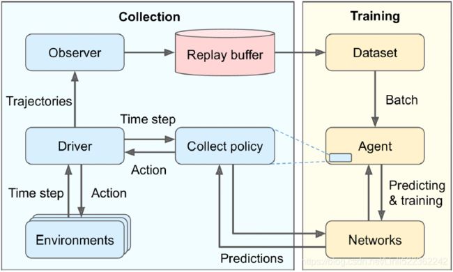
Figure 18-13. A typical TF-Agents training architecture
This figure begs a few questions, which I’ll attempt to answer here:
- • Why are there multiple environments? Instead of exploring a single environment, you generally want the driver to explore multiple copies of the environment in parallel, taking advantage of the power of all your CPU cores, keeping the training GPUs busy, and providing less-correlated trajectories to the training algorithm.
- • What is a trajectory? It is a concise representation of a transition from one time step( including: reward, discount, step_type, observation) to the next, or a sequence of consecutive transitions from time step n to time step n + t. The trajectories collected by the driver are passed to the observer, which saves them in the replay buffer, and they are later sampled by the agent and used for training.
- • Why do we need an observer? Can’t the driver save the trajectories directly? Indeed, it could, but this would make the architecture less flexible.
For example, what if you don’t want to use a replay buffer? What if you want to use the trajectories for something else, like computing metrics? In fact, an observer is just any function that takes a trajectory as an argument. You can use an observer
to save the trajectories to a replay buffer, or
to save them to a TFRecord file (see Cp13 https://blog.csdn.net/Linli522362242/article/details/107704824), or
to compute metrics, or
for anything else.
Moreover, you can pass multiple observers to the driver, and it will broadcast the trajectories to all of them.
Although this architecture is the most common, you can customize it as you please, and even replace some components with your own. In fact, unless you are researching new RL algorithms, you will most likely want to use a custom environment for your task. For this, you just need to create a custom class that inherits from the PyEnvironment class in the tf_agents.environments.py_environment package and overrides the appropriate methods, such as action_spec(), observation_spec(), _reset(), and _step() ( https://towardsdatascience.com/creating-a-custom-environment-for-tensorflow-agent-tic-tac-toe-example-b66902f73059).
###################################################
Creating a Custom TF-Agents Environment
To create a custom TF-Agent environment, you just need to write a class that inherits from the PyEnvironment class and implements a few methods.
For example, the following minimal environment represents a simple 4x4 grid. The agent starts in one corner (0,0) and must move to the opposite corner对角 (3,3). The episode is done if the agent reaches the goal (it gets a +10 reward) or if the agent goes out of bounds (-1 reward). The actions are up (0), down (1), left (2) and right (3).
import tf_agents

class MyEnvironment( tf_agents.environments.py_environment.PyEnvironment ):
  def __init__( self, discount=1.0 ):
    super().__init__()
    self._action_spec = array_spec.BoundedArraySpec(
                                                          shape = (),
                                                          dtype = np.int32,
                                                          name = 'action',
                                                          minimum = 0,
                                                          maximum = 3
                                                        )
    self._observation_spec = array_spec.BoundedArraySpec( shape = (4,4),
                                                               dtype = np.int32,
                                                               name = 'observation',
                                                               minimum = 0,
                                                               maximum = 1
                                                             )
    self.discount = discount

  def action_spec( self ):
    return self._action_spec

  def observation_spec( self ):
    return self._observation_spec

  def _reset( self ):
    self._state = np.zeros( 2, dtype=np.int32 )
    obs = np.zeros( (4,4), dtype=np.int32 )
    obs[ self._state[0], self._state[1] ] = 1
    return tf_agents.trajectories.time_step.restart( obs )
           # Returns a TimeStep with step_type set equal to StepType.FIRST.
           # tf_agents.trajectories.StepType
           #                        Defines the status of a TimeStep within a sequence.
           # FIRST	Instance of numpy.ndarray
           # LAST	Instance of numpy.ndarray
           # MID	Instance of numpy.ndarray

  def _step( self, action ):
              # index:  0       1      2       3
    self._state += [ (-1,0), (+1,0), (0,-1), (0,+1) ][action]
    reward = 0
    obs = np.zeros( (4,4), dtype=np.int32 )
    done = ( self._state.min() < 0 or self._state.max() > 3 )

    if not done:
      obs[ self._state[0], self._state[1] ] = 1

    if done or np.all( self._state == np.array([3,3]) ):
      reward = -1 if done else +10
      return tf_agents.trajectories.time_step.termination( obs, reward )
             # Returns a TimeStep with step_type set to StepType.LAST.
    else:
      return tf_agents.trajectories.time_step.transition( obs, reward, self.discount )
             # Returns a TimeStep with step_type set equal to StepType.MID.
The action and observation specs will generally be instances of the ArraySpec or BoundedArraySpec classes from the tf_agents.specs package (check out the other specs in this package as well). Optionally, you can also define a render() method, a close() method to free resources, as well as a time_step_spec() method if you don't want the reward and discount to be 32-bit float scalars. Note that the base class takes care of keeping track of the current time step, which is why we must implement _reset() and _step() rather than reset() and step().
my_env = MyEnvironment()

time_step = my_env.reset()
time_step
time_step = my_env.step( 1 )
time_step 
###################################################
Now we will create all these components:
- first the Deep Q-Network,
- then the DQN agent (which will take care of creating the collect policy),
- then the replay buffer and the observer to write to it,
- then a few training metrics,
- then the driver, and
- finally the dataset.
- Once we have all the components in place, we will populate the replay buffer with some initial trajectories, then we will run the main training loop. So, let’s start by creating the Deep Q-Network.
Creating the Deep Q-Network
The TF-Agents library provides many networks in the tf_agents.networks package and its subpackages. We will use the tf_agents.networks.q_network.QNetwork class:
Create a small class to normalize the observations. Images are stored using bytes from 0 to 255 to use less RAM, but we want to pass floats from 0.0 to 1.0 to the neural network:
Create the Q-Network:
This QNetwork takes an observation((84, 84, 4)) as input and outputs one Q-Value per action, so we must give it the specifications of the observations(tf_env.observation_spec()) and the actions(tf_env.action_spec()).
###############
Conveniently, a TF-Agents environment provides the specifications of the observations, actions, and time steps, including their shapes, data types, and names, as well as their minimum and maximum values:
env.observation_spec()![]() Observations vary depending on the environment. In this case it is an RGB image represented as a 3D NumPy array of shape [width, height, channels] (with 3 channels: Red, Green and Blue).
Observations vary depending on the environment. In this case it is an RGB image represented as a 3D NumPy array of shape [width, height, channels] (with 3 channels: Red, Green and Blue).
env.action_spec() ![]()
env.time_step_spec()
As you can see, the observations are simply screenshots of the Atari screen, represented as NumPy arrays of shape [210, 160, 3]. To render an environment, you can call env.render(mode="human"), and if you want to get back the image in the form of a NumPy array, just call env.render(mode="rgb_array") (unlike in OpenAI Gym, this is the default mode).
###############
- It starts with a preprocessing layer: a simple Lambda layer that casts the observations to 32-bit floats and normalizes them (the values will range from 0.0 to 1.0).
The observations contain unsigned bytes, which use 4 times less space than 32-bit floats, which is why we did not cast the observations to 32-bit floats earlier; we want to save RAM in the replay buffer. - Next, the network applies three convolutional layers:
the first has 32 8 × 8 filters and uses a stride of 4,
the second has 64 4 × 4 filters and a stride of 2, and
the third has 64 3 × 3 filters and a stride of 1. - Lastly, it applies a dense layer with 512 units, followed by a dense output layer with 4 units, one per Q-Value to output (i.e., one per action, actions=['NOOP', 'FIRE', 'RIGHT', 'LEFT']). All convolutional layers and all dense layers except the output layer use the ReLU activation function by default (you can change this by setting the activation_fn argument). The output layer does not use any activation function.
- https://www.tensorflow.org/agents/api_docs/python/tf_agents/networks/q_network/QNetwork
https://github.com/tensorflow/agents/blob/v0.8.0/tf_agents/networks/q_network.py#L43-L149tf_agents.networks.q_network.QNetwork( input_tensor_spec, action_spec, preprocessing_layers=None, preprocessing_combiner=None, conv_layer_params=None, fc_layer_params=(75, 40), dropout_layer_params=None, activation_fn=tf.keras.activations.relu, kernel_initializer=None, batch_squash=True, dtype=tf.float32, name='QNetwork' )encoder = encoding_network.EncodingNetwork( encoder_input_tensor_spec, preprocessing_layers=preprocessing_layers, preprocessing_combiner=preprocessing_combiner, conv_layer_params=conv_layer_params, fc_layer_params=fc_layer_params, dropout_layer_params=dropout_layer_params, activation_fn=activation_fn, kernel_initializer=kernel_initializer, batch_squash=batch_squash, dtype=dtype) q_value_layer = tf.keras.layers.Dense( num_actions, activation=None, kernel_initializer=tf.random_uniform_initializer( minval=-0.03, maxval=0.03), bias_initializer=tf.constant_initializer(-0.2), dtype=dtype)
from tf_agents.networks.q_network import QNetwork
from tensorflow import keras

preprocessing_layer = keras.layers.Lambda( lambda obs:
                                              tf.cast( obs, np.float32 )/ 255. )
conv_layer_params = [ (32, (8,8), 4), # 32, 8 × 8 filter, strides = 4
                      (64, (4,4), 2),
                      (64, (3,3), 1)
                    ]
fc_layer_params = [512] # a dense layer with 512 units

q_net = QNetwork( tf_env.observation_spec(),
                  tf_env.action_spec(),
                  preprocessing_layers = preprocessing_layer,
                  conv_layer_params = conv_layer_params,
                  fc_layer_params = fc_layer_params
                )
Under the hood, a QNetwork is composed of two parts:
- an encoding network that processes the observations, followed by a dense output layer that outputs one Q-Value per action(actions=['NOOP', 'FIRE', 'RIGHT', 'LEFT']).
- TF-Agent’s EncodingNetwork class implements a neural network architecture found in various agents (see Figure 18-14).

Figure 18-14. Architecture of an encoding network
It may have one or more inputs. For example, if each observation is composed of some sensor data plus an image from a camera, you will have two inputs. Each input may require some preprocessing steps, in which case you can specify a list of Keras layers via the preprocessing_layers argument, with one preprocessing layer per input, and the network will apply each layer to the corresponding input (if an input requires multiple layers of preprocessing, you can pass a whole model, since a Keras model can always be used as a layer). If there are two inputs or more, you must also pass an extra layer via the preprocessing_combiner argument, to combine the outputs from the preprocessing layers into a single output.
Next, the encoding network will optionally apply a list of convolutions sequentially, provided you specify their parameters via the conv_layer_params argument. This must be a list composed of 3-tuples (one per convolutional layer) indicating the number of filters, the kernel size, and the stride. After these convolutional layers, the encoding network will optionally apply a sequence of dense layers, if you set the fc_layer_params argument: it must be a list containing the number of neurons for each dense layer. Optionally, you can also pass a list of dropout rates (one per dense layer) via the dropout_layer_params argument if you want to apply dropout after each dense layer. The QNetwork takes the output of this encoding network and passes it to the dense output layer (with one unit per action).
The QNetwork class is flexible enough to build many different architectures, but you can always build your own network class if you need extra flexibility: extend the tf_agents.networks.Network class and implement it like a regular custom Keras layer. The tf_agents.networks.Network class is a subclass of the keras.layers.Layer class that adds some functionality required by some agents, such as the possibility to easily create shallow copies浅层副本 of the network (i.e., copying the network’s architecture, but not its weights). For example, the DQNAgent uses this to create a copy of the online model.
Now that we have the DQN, we are ready to build the DQN agent.
Creating the DQN Agent
The TF-Agents library implements many types of agents, located in the tf_agents.agents package and its subpackages. We will use the tf_agents.agents.dqn.dqn_agent.DqnAgent class:
Let’s walk through this code:
- • We first create a variable that will count the number of training steps.
train_step = tf.Variable(0)
- • Then we build the optimizer, using the same hyperparameters as in the 2015 DQN paper.https://arxiv.org/pdf/1509.06461.pdf
The optimization employed to train the network is RMSProp (with momentum parameter 0.95, rho; the learning rate to α = 0.00025; epsilon = 0.00001).
- • Next, we create a PolynomialDecay object that will compute the ε value for the ε-greedy collect policy, given the current training step (it is normally used to decay the learning rate, hence the names of the arguments, but it will work just fine to decay any other value). It will go from 1.0 down to 0.01 (the value used during in the 2015 DQN paper) in 1 million ALE frames, which corresponds to 250,000 steps = 1 million // 4, since we use frame skipping with a period of 4(1 step = 4 frames). Moreover, we will train the agent every 4 steps (i.e., 16 ALE frames), so ε will actually decay over 62,500 training steps = 250,000 steps // update_period.
https://github.com/tensorflow/agents/blob/master/tf_agents/agents/dqn/dqn_agent.py - • We then build the DQNAgent, passing it
the time step # tf_env.time_step_spec(),
and action specs, # tf_env.action_spec(),
the QNetwork to train, # q_network = q_net,
the optimizer, # types.Optimizer
the number of training steps between target model updates (τ=2000, 2000*16=32,000 ale frames), # target_update_period = 2000
the loss function to use, # td_errors_loss_fn = keras.losses.Huber( reduction="none" ),
the discount factor, # gamma = 0.99,
the train_step variable(train_step_counter = train_step), and
a function that returns the ε value (it must take no argument, which is why we need a lambda to pass the train_step, epsilon_greedy = lambda: epsilon_fn( train_step )). Note that the loss function must return an error per instance, not the mean error, which is why we set reduction="none".
epsilon_greedy: probability of choosing a random action in the default epsilon-greedy collect policy (used only if a wrapper is not provided to the collect_policy method). Only one of epsilon_greedy and boltzmann_temperature should be provided. - • Lastly, we initialize the agent.
from tf_agents.agents.dqn.dqn_agent import DqnAgent

train_step = tf.Variable(0)
update_period = 4                   # run a training step every 4 collect steps

# https://blog.csdn.net/Linli522362242/article/details/106982127
# https://keras.io/api/optimizers/rmsprop/
optimizer = keras.optimizers.RMSprop( learning_rate=2.5e-4,
                                      rho = 0.95, # Discounting factor for the history/coming gradient. Defaults to 0.9.
                                      momentum = 0.0,
                                      epsilon = 0.00001,
                                      centered = True # Boolean. If True, gradients are normalized by the estimated variance of the gradient;
                                    )
epsilon_fn = keras.optimizers.schedules.PolynomialDecay(
                                                        initial_learning_rate = 1.0, # initial e
                                                        decay_steps = 250000//update_period, # <=> 1,000,000 ALE frames
                                                        end_learning_rate = 0.01    # final e
                                                       )

# https://github.com/tensorflow/agents/blob/master/tf_agents/agents/dqn/dqn_agent.py
agent = DqnAgent( tf_env.time_step_spec(),
                  tf_env.action_spec(),
                  q_network = q_net,
                  optimizer = optimizer,
                  target_update_period = 2000, # ==> 32,000 ALE frames since 1 step = 4 frames, train the agent every 4 steps
                  td_errors_loss_fn = keras.losses.Huber( reduction="none" ),
                  gamma = 0.99,                # discount factor
                  train_step_counter = train_step,
                  epsilon_greedy = lambda: epsilon_fn( train_step )
                )
agent.initialize()
Next, let’s build the replay buffer and the observer that will write to it.
Creating the Replay Buffer and the Corresponding Observer
The TF-Agents library provides various replay buffer implementations in the tf_agents.replay_buffers package. Some are purely written in Python (their module names start with py_), and others are written based on TensorFlow (their module names start with tf_). We will use the TFUniformReplayBuffer class in the tf_agents.replay_buffers.tf_uniform_replay_buffer package. It provides a high-performance implementation of a replay buffer with uniform sampling: https://github.com/tensorflow/agents/blob/master/tf_agents/replay_buffers/tf_uniform_replay_buffer.py
    The TFUniformReplayBuffer stores episodes in `B == batch_size` blocks of
    size `L == max_length`, with total frame capacity
    `C == L * B`.  Storage looks like:
    ```
    block1 ep1 frame1
               frame2
           ...
           ep2 frame1
               frame2
           ...

    block2 ep1 frame1
               frame2
           ...
           ep2 frame1
               frame2
           ...

    ...
    blockB ep1 frame1
               frame2
           ...
           ep2 frame1
               frame2
           ...

    ```
    Multiple episodes may be stored within a given block, up to `max_length`
    frames total.  In practice, new episodes will overwrite old ones as the
    block rolls over its `max_length`.
Let’s look at each of arguments:
- data_spec # A TensorSpec or a list/tuple/nest of TensorSpecs describing a single item that can be stored in this buffer.
The specification of the data that will be saved in the replay buffer. The DQN agent knowns what the collected data will look like, and it makes the data spec available via its collect_data_spec attribute, so that’s what we give the replay buffer.
- batch_size # Batch dimension of tensors when adding to buffer.
The number of trajectories that will be added at each step. In our case, it will be one, since the driver will just execute one action per step and collect one trajectory.
If the environment were a batched environment, meaning an environment that takes a batch of actions at each step and returns a batch of observations, then the driver would have to save a batch of trajectories at each step. Since we are using a TensorFlow replay buffer, it needs to know the size of the batches it will handle (to build the computation graph).
An example of a batched environment is the ParallelPyEnvironment (from the tf_agents.environments.parallel_py_environment package): it runs multiple environments in parallel in separate processes (they can be different as long as they have the same action and observation specs), and at each step it takes a batch of actions and executes them in the environments (one action per environment), then it returns all the resulting observations.
- max_length # The maximum number of items that can be stored in a single batch segment of the buffer.
The maximum size of the replay buffer. We created a large replay buffer that can store one million trajectories (as was done in the 2015 DQN paper). This will require a lot of RAM.
Create the replay buffer (this will use a lot of RAM, so please reduce the buffer size if you get an out-of-memory error):
Warning: we use a replay buffer of size 100,000 instead of 1,000,000 (as used in the book) since many people were getting OOM (Out-Of-Memory, colab ram=12.65GB ) errors.
https://www.tensorflow.org/agents/api_docs/python/tf_agents/agents/TFAgent
collect_data_spec: Property that describes the structure expected of experience collected by agent.collect_policy. This is typically identical to training_data_spec, but may be different if preprocess_sequence method is not the identity. In this case, preprocess_sequence is expected to read sequences matching collect_data_spec and emit sequences matching training_data_spectf_env.batch_size
from tf_agents.replay_buffers import tf_uniform_replay_buffer

replay_buffer = tf_uniform_replay_buffer.TFUniformReplayBuffer(
                                            data_spec = agent.collect_data_spec,
                                            batch_size = tf_env.batch_size,
                                            max_length = 100000 # # reduce if OOM error
                )
replay_buffer_observer = replay_buffer.add_batch
Now we can create the observer that will write the trajectories to the replay buffer. An observer is just a function (or a callable object) that takes a trajectory argument, so we
can directly use the add_method() method (bound to the replay_buffer object) as our observer : replay_buffer_observer = replay_buffer.add_batch
When we store two consecutive trajectories, they contain two consecutive observations with four frames each (since we used the FrameStack4 wrapper), and unfortunately three of the four frames in the second observation are redundant (they are already present in the first observation). In other words, we are using about four times more RAM than necessary. To avoid this, you can instead use a PyHashedReplayBuffer from the tf_agents.replay_buffers.py_hashed_replay_buffer package: it deduplicates data in the stored trajectories along the last axis of the observations
If you wanted to create your own observer, you could write any function with a trajectory argument. If it must have a state, you can write a class with a __call__(self, trajectory) method.
For example, here is a simple observer that will increment a counter every time it is called (except when the trajectory represents a boundary between two episodes, which does not count as a step), and every 100 increments it displays the progress up to a given total (the carriage return \r along with end="" ensures that the displayed counter remains on the same line):
  def is_boundary(self) -> types.Bool:
    if tf.is_tensor(self.step_type):
      return tf.equal(self.step_type, ts.StepType.LAST)
    return self.step_type == ts.StepType.LAST
https://github.com/tensorflow/agents/blob/v0.8.0/tf_agents/trajectories/trajectory.py#L395-L429
A sampled trajectory may actually overlap two (or more) episodes! In this case, it will contain boundary transitions, meaning transitions with a step_type equal to 2 (end) and a next_step_type equal to 0 (start). Of course, TF-Agents properly handles such trajectories (e.g., by resetting the policy state when encountering a boundary). The trajectory’s is_boundary() method returns a tensor indicating whether each step is a boundary or not.
class ShowProgress:
  def __init__( self, total ):
    self.counter = 0
    self.total = total

  def __call__( self, trajectory ):
    if not trajectory.is_boundary():
      self.counter +=1
    if self.counter % 100 == 0:
      print( "\r{}/{}".format(self.counter, self.total), end="" )
Now let’s create a few training metrics.
Creating Training Metrics
TF-Agents implements several RL metrics in the tf_agents.metrics package, some purely in Python and some based on TensorFlow. Let’s create a few of them in order to count the number of episodes, the number of steps taken, and most importantly the average return per episode and the average episode length:
from tf_agents.metrics import tf_metrics

train_metrics = [
                  tf_metrics.NumberOfEpisodes(),           # count the number of episodes
                  tf_metrics.EnvironmentSteps(),           # the number of steps taken
                  tf_metrics.AverageReturnMetric(),        # the average return per episode
                  tf_metrics.AverageEpisodeLengthMetric(), # the average episode length
                ]
Discounting the rewards makes sense for training or to implement a policy, as it makes it possible to balance the importance of immediate rewards with future rewards. However, once an episode is over, we can evaluate how good it was overalls by summing the undiscounted rewards. For this reason, the AverageReturnMetric computes the sum of undiscounted rewards for each episode, and it keeps track of the streaming mean of these sums over all the episodes it encounters.
train_metrics[0].result()![]()
At any time, you can get the value of each of these metrics by calling its result() method (e.g., train_metrics[0].result()).
Alternatively, you can log all metrics by calling log_metrics(train_metrics) (this function is located in the tf_agents.eval.metric_utils package):
from tf_agents.eval.metric_utils import log_metrics
import logging

logging.getLogger().setLevel( logging.INFO )
log_metrics( train_metrics ) 
Next, let’s create the collect driver.
Creating the Collect Driver
Figure 18-13
As we explored in Figure 18-13, a driver is an object that explores an environment using a given policy, collects experiences, and broadcasts them to some observers. At each step, the following things happen:
- • The driver passes the current time step to the collect policy, which uses this time step to choose an action and returns an action step object containing the action.
- • The driver then passes the action to the environment, which returns the next time step.
- • Finally, the driver creates a trajectory object to represent this transition and broadcasts it to all the observers.
Some policies, such as RNN policies, are stateful(https://blog.csdn.net/Linli522362242/article/details/115388298): they choose an action based on both the given time step and their own internal state. Stateful policies return their own state in the action step, along with the chosen action.
The driver will then pass this state back to the policy at the next time step. Moreover, the driver saves the policy state to the trajectory (in the policy_info field), so it ends up in the replay buffer.
This is essential when training a stateful policy: when the agent samples a trajectory, it must set the policy’s state to the state it was in at the time of the sampled time step.
Also, as discussed earlier, the environment may be a batched environment, in which case the driver passes a batched time step to the policy (i.e., a time step object containing
- a batch of observations,
- a batch of step types,
- a batch of rewards, and
- a batch of discounts,
- all 4 batches of the same size).
The driver also passes a batch of previous policy states.
The policy then returns a batched action step containing
- a batch of actions and
- a batch of policy states.
Finally, the driver creates a batched trajectory (i.e., a trajectory containing
- a batch of step types,
- a batch of observations,
- a batch of actions,
- a batch of rewards, and
- more generally a batch for each trajectory attribute, with all batches of the same size).
There are two main driver classes: DynamicStepDriver and DynamicEpisodeDriver. The first one collects experiences for a given number of steps, while the second collects experiences for a given number of episodes. We want to collect experiences for 4 steps for each training iteration (as was done in the 2015 DQN paper), so let’s create a DynamicStepDriver:
from tf_agents.drivers.dynamic_step_driver import DynamicStepDriver

collect_driver = DynamicStepDriver(
                                    tf_env, # tf_env = TFPyEnvironment( env ) # env = suite_atari.load(...)
                                    agent.collect_policy,     # epsilon_greedy
                                    observers = [replay_buffer_observer] + train_metrics,
                                    num_steps = update_period # collect 4 steps for each training iteration
                                  )
We give it
- the environment to play with,
- the agent’s collect policy,
- a list of observers (including the replay buffer observer and the training metrics),
- and finally the number of steps to run (in this case, 4 since we train the agent every 4 steps).
num_steps: The number of steps to take in the environment. For batched or parallel environments, this is the total number of steps taken summed across all environments.
We could now run it by calling its run() method, but it’s best to warm up the replay buffer with experiences collected using a purely random policy. For this, we can use the RandomTFPolicy class and create a second driver that will run this policy for 20,000 steps (which is equivalent to 80,000 simulator frames(since 1 step = 4 frames), as was done in the 2015 DQN paper). We can use our ShowProgress observer to display the progress:
Collect the initial experiences, before training:
from tf_agents.policies.random_tf_policy import RandomTFPolicy

initial_collect_policy = RandomTFPolicy( tf_env.time_step_spec(),
                                         tf_env.action_spec()
                                       )
init_driver = DynamicStepDriver(
                                  tf_env, # tf_env = TFPyEnvironment( env ) # env = suite_atari.load(...)
                                  initial_collect_policy,
                                  observers = [replay_buffer.add_batch, ShowProgress(20000)],
                                  num_steps = 20000 # ==80,000 ALE frame since 1 step = 4 frames
                               )
final_time_step, final_policy_state = init_driver.run()
We’re almost ready to run the training loop! We just need one last component: the dataset.
Creating the Dataset
To sample a batch of trajectories from the replay buffer, call its get_next() method. This returns the batch of trajectories plus a BufferInfo object that contains the sample identifiers and their sampling probabilities (this may be useful for some algorithms, such as PER).
For example, the following code will sample a small batch of two trajectories (subepisodes, sample_batch_size=2), each containing 3 consecutive steps(num_steps=3). These subepisodes are shown in Figure 18-15 (each row contains three consecutive steps from an episode):
Note: replay_buffer.get_next() is deprecated. We must use replay_buffer.as_dataset(..., single_deterministic_pass=False) instead.
tf.random.set_seed(9) # chosen to show an example of trajectory at the end of an episode

#trajectories, buffer_info = replay_buffer.get_next( # get_next() is deprecated
#    sample_batch_size=2, num_steps=3)

trajectories, buffer_info = next( iter( replay_buffer.as_dataset( sample_batch_size=2,
                                                                  num_steps=3,
                                                                  single_deterministic_pass=False
                                                                )
                                      )
                                )
trajectories._fields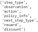
trajectories.observation.shape ![]()
trajectories.step_type.numpy() ![]()
The trajectories object is a named tuple, with 7 fields. Each field contains a tensor whose first two dimensions are 2 and 3 (since there are 2 trajectories, each with 3 steps). This explains why the shape of the observation field is [2, 3, 84, 84, 4]: that’s two trajectories, each with three steps, and each step’s observation is 84 × 84 × 4. Similarly, the step_type tensor has a shape of [2, 3]: in this example, both trajectories contain 3 consecutive steps in the middle on an episode (types 1, 1, 1).
The step_type attribute is equal to
- 0 for the first time step in the episode,
- 1 for intermediate time steps, and
- 2 for the final time step.
from tf_agents.trajectories.trajectory import to_transition

time_steps, action_steps, next_time_steps = to_transition( trajectories )
time_steps.observation.shape![]() The to_transition() function in the tf_agents.trajectories.trajectory module converts a batched trajectory(The trajectories object is a named tuple, with 7 fields) into a list containing a batched time_step (step_types, observations), a batched action_step(actions, policy_infos), and a batched next_time_step(rewards, discounts, step_types). Notice that the second dimension is 2 instead of 3, since there are t transitions between t + 1 time steps (don’t worry if you’re a bit confused; 2 steps = 1 full transition):
The to_transition() function in the tf_agents.trajectories.trajectory module converts a batched trajectory(The trajectories object is a named tuple, with 7 fields) into a list containing a batched time_step (step_types, observations), a batched action_step(actions, policy_infos), and a batched next_time_step(rewards, discounts, step_types). Notice that the second dimension is 2 instead of 3, since there are t transitions between t + 1 time steps (don’t worry if you’re a bit confused; 2 steps = 1 full transition):
trajectories.step_type.numpy() ![]()
def plot_observation( obs ):
    obs = obs.astype( np.float32 )
    img = obs[..., :3]                # 3th frame
    current_frame_delta = np.maximum( obs[..., 3] - obs[..., :3].mean( axis=-1),
                                      0.
                                    )
    img[..., 0] += current_frame_delta # red
    img[..., 2] += current_frame_delta # blue
    img = np.clip( img/150, 0, 1)

    plt.imshow( img )
    plt.axis('off')

plt.figure( figsize=(10, 6.8) )

for row in range(2):
  for col in range(3):
    plt.subplot( 2,3, row*3 + col +1 )
    plot_observation( trajectories.observation[row, col].numpy() )

plt.subplots_adjust( left=0, right=1, bottom=0, top=1, hspace=0, wspace=0.02 )

plt.show()
In the second trajectory, you can barely see the ball![]() at the lower left of the first observation, and it disappears in the next two observations, so the agent is about to lose a life, but the episode will not end immediately because it still has several lives left.
at the lower left of the first observation, and it disappears in the next two observations, so the agent is about to lose a life, but the episode will not end immediately because it still has several lives left.
Figure 18-15. Two trajectories containing three consecutive steps each


Figure 18-16. Trajectories, transitions, time steps, and action steps
Each trajectory is a concise representation of a sequence of consecutive time steps and action steps, designed to avoid redundancy. How so? Well, as you can see in Figure 18-16, transition n is composed of time step n, action step n, and time step n + 1, while transition n + 1 is composed of time step n + 1, action step n + 1, and time step n + 2. If we just stored these two transitions directly in the replay buffer, the time step n + 1(reward, discount, step_type, observation) would be duplicated.
To avoid this duplication, the n_th trajectory step includes only the step_type and observation from time step n (not its reward and discount), and it does not contain the observation from time step n + 1 (however, it does contain a copy of the next time step’s type; that’s the only duplication).
So if you have a batch of trajectories where each trajectory has 1+t steps (from time step n to time step n + t), then it contains all the data from time step n to time step n + t, except for the reward and discount from time step n (only the step_type and observation from time step n) (but it contains the reward, discount and a copy of step_type of time step n + t + 1). This represents t transitions (n to n + 1, n + 1 to n + 2, …, n + t – 1 to n + t).
For our main training loop, instead of calling the get_next() method, we will use a tf.data.Dataset. This way, we can benefit from the power of the Data API (e.g., parallelism and prefetching). For this, we call the replay buffer’s as_dataset() method:
dataset = replay_buffer.as_dataset(
                                    sample_batch_size = 64,
                                    num_steps = 2,
                                    num_parallel_calls = 3
                                  ).prefetch(3)
We will sample batches of 64 trajectories at each training step (as in the 2015 DQN paper), each with 2 steps (i.e., 2 steps = 1 full transition, including the next step’s observation). This dataset will process three elements in parallel, and prefetch three batches.
For on-policy algorithms such as Policy Gradients, each experience should be sampled once, used from training, and then discarded. In this case, you can still use a replay buffer, but instead of using a Dataset, you would call the replay buffer’s gather_all() method at each training iteration to get a tensor containing all the trajectories recorded so far, then use them to perform a training step, and finally clear the replay buffer by calling its clear() method.
Now that we have all the components in place, we are ready to train the model!
Creating the Training Loop
To speed up training, we will convert the main functions to TensorFlow Functions. For this we will use the tf_agents.utils.common.function() function, which wraps tf.function(), with some extra experimental options:
from tf_agents.utils.common import function

collect_driver.run = function( collect_driver.run )
agent.train = function( agent.train)
Let’s create a small function that will run the main training loop for n_iterations:
The function
- first asks the collect policy for its initial state (given the environment batch size, which is 1 in this case). Since the policy is stateless, this returns an empty tuple (so we could have written policy_state = ()).
- Next, we create an iterator over the dataset
and we run the training loop. At each iteration, we call the driver’s run() method, passing it the current time step (initially None) and the current policy state. # collect_driver.run( time_step, policy_state )
It will run the collect policy and collect experience for 4 steps (as we configured earlier, num_steps = update_period # collect 4 steps for each training iteration), broadcasting the collected trajectories to the replay buffer and the metrics(observers = [replay_buffer_observer] + train_metrics).
Next, we sample one batch of trajectories from the dataset, #trajectories, buffer_info = next( iterator )
and we pass it to the agent’s train() method. It returns a train_loss object which may vary depending on the type of agent.
# train_loss = agent.train( trajectories )
Next, we display the iteration number and the training loss, and every 1,000 iterations we log all the metrics.
def train_agent( n_iterations ):
  time_step = None                                     # tf_env.batch_size ==1
  policy_state = agent.collect_policy.get_initial_state( tf_env.batch_size )
  iterator = iter( dataset )

  for iteration in range( n_iterations ):
    time_step, policy_state = collect_driver.run( time_step, policy_state )
    trajectories, buffer_info = next( iterator )
    train_loss = agent.train( trajectories )

    print( "\r{} loss:{:.5f}".format( iteration, train_loss.loss.numpy() ),
          end="" )
    if iteration % 1000 == 0:
      log_metrics( train_metrics )
Now you can just call train_agent() for some number of iterations, and see the agent gradually learn to play Breakout!
Run the next cell to train the agent for 30,000 steps. Then look at its behavior by running the following cell. You can run these two cells as many times as you wish. The agent will keep improving! It will likely take over 200,000 iterations for the agent to become reasonably good.
train_agent( n_iterations=30000 )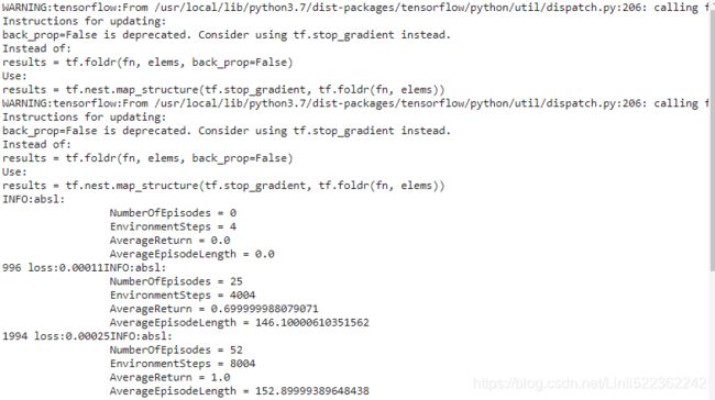
from IPython import display as ipythondisplay
from pyvirtualdisplay import Display

import matplotlib.animation as animation
import matplotlib as mpl
mpl.rc('animation', html='jshtml')

def update_scene( num, frames, patch ):
    patch.set_data( frames[num] )
    return patch,

def plot_animation( frames, repeat=False, interval=40 ):
    fig = plt.figure()
    patch = plt.imshow( frames[0] ) # img
    plt.axis( 'off' )


    anim = animation.FuncAnimation(
            fig,         # figure
            func=update_scene, # The function to call at each frame.
            fargs=(frames, patch), # Additional arguments to pass to each call to func.
            frames = len(frames),  # iterable, int, generator function, or None, optional : Source of data to pass func and each frame of the animation
            repeat=repeat,
            interval=interval
    )
    plt.close()
    return anim
frames = []
def save_frames( trajectory ):
global frames
frames.append( tf_env.pyenv.envs[0].render(mode="rgb_array") )
watch_driver = DynamicStepDriver(
tf_env,
agent.policy,
observers = [ save_frames, ShowProgress(1000) ],
num_steps = 1000
)
final_time_step, final_policy_state = watch_driver.run()
plot_animation(frames) 
import PIL
import os

image_path = os.path.join("/content/drive/MyDrive/hand_on_ml/", "breakout.gif")
frame_images = [ PIL.Image.fromarray(frame) for frame in frames[:150] ]
frame_images[0].save( image_path, format='GIF',
                      append_images=frame_images[1:],
                      save_all=True,
                      duration=30,
                      loop=0
                     )
This will take a lot of computing power and a lot of patience (it may take hours, or even days, depending on your hardware), plus you may need to run the algorithm several times with different random seeds to get good results, but once it’s done, the agent will be superhuman (at least at Breakout). You can also try training this DQN agent on other Atari games: it can achieve superhuman skill at most action games, but it is not so good at games with long-running storylines. (For a comparison of this algorithm’s performance on various Atari games, see figure 3 in DeepMind’s 2015 paper.)
Overview of Some Popular RL Algorithms
Before we finish this chapter, let’s take a quick look at a few popular RL algorithms:
- Actor-Critic algorithms
A family of RL algorithms that combine Policy Gradients with Deep QNetworks. An Actor-Critic agent contains two neural networks: a policy net and a DQN.
The DQN is trained normally, by learning from the agent’s experiences.
The policy net learns differently (and much faster) than in regular PG: instead of estimating the value of each action by going through multiple episodes, then summing the future discounted rewards for each action, and finally normalizing them,
the agent (actor) relies on the action values estimated by the DQN (critic). It’s a bit like an athlete (the agent) learning with the help of a coach (the DQN).
- Asynchronous Advantage Actor-Critic (A3C) (Volodymyr Mnih et al., “Asynchonous Methods for Deep Reinforcement Learning,” Proceedings of the 33rd International Conference on Machine Learning (2016): 1928–1937.)
An important Actor-Critic variant introduced by DeepMind researchers in 2016, where multiple agents learn in parallel, exploring different copies of the environment. At regular intervals, but asynchronously (hence the name), each agent pushes some weight updates to a master network, then it pulls the latest weights from that network. Each agent thus contributes to improving the master network and benefits from what the other agents have learned. Moreover, instead of estimating the Q-Values, the DQN estimates the advantage of each action (hence the second A in the name), which stabilizes training.
- Advantage Actor-Critic (A2C)
A variant of the A3C algorithm that removes the asynchronicity. All model updates are synchronous, so gradient updates are performed over larger batches, which allows the model to better utilize the power of the GPU.
- Soft Actor-Critic (SAC) (Tuomas Haarnoja et al., “Soft Actor-Critic: Off-Policy Maximum Entropy Deep Reinforcement Learning with a Stochastic Actor,” Proceedings of the 35th International Conference on Machine Learning (2018): 1856–1865.)
An Actor-Critic variant proposed in 2018 by Tuomas Haarnoja and other UC Berkeley researchers. It learns not only rewards, but also to maximize the entropy of its actions. In other words, it tries to be as unpredictable as possible while still getting as many rewards as possible. This encourages the agent to explore the environment, which speeds up training, and makes it less likely to repeatedly execute the same action when the DQN produces imperfect estimates. This algorithm has demonstrated an amazing sample efficiency (contrary to all the previous algorithms, which learn very slowly). SAC is available in TF-Agents.
- Proximal Policy Optimization近端策略优化 (PPO)(John Schulman et al., “Proximal Policy Optimization Algorithms,” arXiv preprint arXiv:1707.06347 (2017).)
An algorithm based on A2C that clips the loss function to avoid excessively large weight updates (which often lead to training instabilities). PPO is a simplification of the previous Trust Region Policy Optimization (TRPO) algorithm(John Schulman et al., “Trust Region Policy Optimization,” Proceedings of the 32nd International Conference on Machine Learning (2015): 1889–1897.), also by John Schulman and other OpenAI researchers. OpenAI made the news in April 2019 with their AI called OpenAI Five, based on the PPO algorithm, which defeated the world champions at the multiplayer game Dota 2. PPO is also available in TF-Agents.
- Curiosity-based exploration(Deepak Pathak et al., “Curiosity-Driven Exploration by Self-Supervised Prediction,” Proceedings of the 34th International Conference on Machine Learning (2017): 2778–2787.)
A recurring problem in RL is the sparsity稀疏性 of the rewards, which makes learning very slow and inefficient. Deepak Pathak and other UC Berkeley researchers have proposed an exciting way to tackle this issue: why not ignore the rewards, and just make the agent extremely curious to explore the environment? The rewards thus become intrinsic固有的 to the agent, rather than coming from the environment. Similarly, stimulating curiosity激发孩子 in a child is more likely to give good results than purely rewarding the child for getting good grades. How does this work? The agent continuously tries to predict the outcome of its actions, and it seeks situations where the outcome does not match its predictions. In other words, it wants to be surprised. If the outcome is predictable (boring), it goes elsewhere. However, if the outcome is unpredictable but the agent notices that it has no control over it, it also gets bored after a while. With only curiosity, the authors succeeded in training an agent at many video games: even though the agent gets no penalty for losing, the game starts over, which is boring so it learns to avoid it.
We covered many topics in this chapter: Policy Gradients, Markov chains, Markov decision processes, Q-Learning, Approximate Q-Learning, and Deep Q-Learning and its main variants (fixed Q-Value targets, Double DQN, Dueling DQN, and prioritized experience replay). We discussed how to use TF-Agents to train agents at scale, and finally we took a quick look at a few other popular algorithms. Reinforcement Learning is a huge and exciting field, with new ideas and algorithms popping out every day, so I hope this chapter sparked your curiosity: there is a whole world to explore!
Exercises
https://blog.csdn.net/Linli522362242/article/details/119267256