Ch4. Least Squares - An Informal Introduction - Sensing and State Estimation II - uni-bonn

之前看bonn大学Cyrill Stachniss教授的课基于图的SLAM中最小二乘求最优的时候提到了Information Matrix。

Information Matrix这个概念以前用最小二乘的时候并没有看见过。

所以回头来看前一章最小二乘的内容。

 

定义

Least Squares 是用在overdetermined system（超定？超验？）里面的。

我们的等式要比变量多。

经常用于给定观测，轨迹模型参数。

 

我们有系统状态X，用一个observation function去估计可能会观察到的observation。

Z是实际观测

Z_hat是预测

我们要做的就是，找到最能让实际观测Z和预测Z_hat最符合的状态X。

我们设定error符合mean = 0 的高斯分布

假设我们还知道我们的sensor有多好，用information matrix Ω表示。

在把error转换成square error的时候，我们把information matrix Ω引入作为weight。

F（X）是所有error的形式，具体可以展开成sum of squared error terms 或者sum of 别的 error terms

正常来说就是求导找极值，当然也有非线性形式要处理。

所以我们需要有一个不错的初始值，还希望我们的error function 比较平滑

最好是全局平滑，别一下自跑到局部最优了。

具体来说，就是在把error局部线性化，然后求一阶导数，设导为0找到极值，或者极值处的状态，开始下一轮迭代。

这里就引入泰勒展开啦来做局部的线性近似化啦。

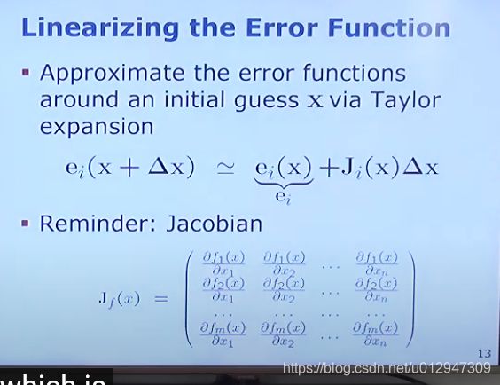
用局部线性化的square error替代原本的squared error

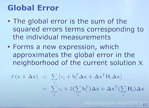
交换一下

可以看到第一个term是consisten，第二个term中间部分用B^T_i替代，最后一个term部分用Hi替代。

其实就是把跟Δx不相关的部分提出来。

写回global error term的样子

具体步骤，写好global error term的quadratic form；

计算一阶导；设一阶导为0；解决；

算导数的时候，consisten部分就kick out了，剩下的好像是根据Derrick term

那x+Δx（假设X为常数，对Δx求导）附近的一阶导怎么样的呢

然后设置为0，解出Δx

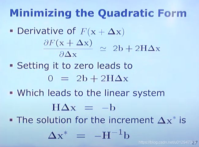
这就是经典的高斯牛顿法了

例子：里程计标定

 （曾书格的激光雷达课程里面刚好有里程计标定作业欸）

假设我们有一个f_i(X)，这个方程可以把有噪声的参数X转换成无偏的输出。

写成state vector，error function 和derivative的形式后（Jocabinan是9列3行，error function 3行，status vector9列。）

注意这里是的jacobian已经没有变量X在里面了，因为这个例子是线性系统，initial guess就没意义了，直接就找到极值了。

Questions

如果odometry是完美的，那parameters自然是Identical拉

至少要3个，每个等式提供三个约束。

H=ΣJ^TΩJ，这不是就是symmetrics嘛

我们的观测越能描述变量，那我们的Jacobian和H就越dense。

HΔx=-b中H矩阵求逆

实际上很多情况H矩阵没法直接求逆，所以我们用这些理论来求H的逆。（我就用过QR分解）

A*X=b

A=L*L^T

L*(L^T*X)=B

L*Y=B (Y是个向量)

Y=L^T*X

好了，融会贯通的大佬才能明白的知识点来了。

最小二乘法和概率状态估计的关系

首先根据贝叶斯理论和马可夫假设，我们有一个the probability of states x(0:t) given observation z(1:t)和control vector u(1:t).

这个probability 可以被重写成 下面的形式 (?????) 

=normalization constant * prior * Π（motion model * observation model）

写成log likelihood形式（累积转累加）然后我们假设这些的term都符合高斯分布

回顾一下高斯likelihood，我们有变量x，均值μ，协方差Σ

我们重新定义(x-μ)^T为，我们定义1/Σ为Ω，x-μ为e(x)

那跟之前的square error 是一样的形状（？？？？？？之前那个的形状？）

把error term插入到之前的log likelihood之后得到下面的式子。

绕口的地方来了，maximizing the probability distribution from maximizing the error terms 

is equivalent to

minimizing the prior plus the error resulting from motion commands and observations

翻译过来就是

我们有一个独立的高斯分布，我们要使它的log likelihood最大，就等于把使得square error最小。（拗口但是好懂）

 

所以这一章没有解释information matrix Ω 和H和b，只是定义了它们。