swin transformer总结
1 原文
论文链接:Swin Transformer: Hierarchical Vision Transformer using Shifted Windows
源码地址:https://github.com/microsoft/Swin-Transformer
2 引言
目前Transformer应用到图像领域主要有两大挑战:
- 视觉实体变化大,在不同场景下视觉Transformer性能未必很好。即目标尺寸多变。不像NLP任务中token大小基本相同,目标检测中的目标尺寸不一,用单层级的模型很难有好的效果。
- 图像分辨率高,像素点多,Transformer基于全局自注意力的计算导致计算量较大。即图片的高分辨率。尤其是在分割任务中,高分辨率会使得计算复杂度呈现输入图片大小的二次方增长,这显然是不能接受的。
针对上述两个问题,我们提出了一种包含滑窗操作,具有层级设计的Swin Transformer。
其中滑窗操作包括不重叠的local window,和重叠的cross-window。将注意力计算限制在一个窗口中,一方面能引入CNN卷积操作的局部性,另一方面能节省计算量。

在各大图像任务上,Swin Transformer都具有很好的性能。
3 整体架构
我们先看下Swin Transformer的整体架构

- 首先将图片输入到Patch Partition模块中进行分块,即每4x4相邻的像素为一个Patch,然后在channel方向展平(flatten)。假设输入的是RGB三通道图片,那么每个patch就有4x4=16个像素,然后每个像素有R、G、B三个值所以展平后是16x3=48,所以通过Patch Partition后图像shape由 [H, W, 3]变成了 [H/4, W/4, 48]。然后在通过Linear Embeding层对每个像素的channel数据做线性变换,由48变成C,即图像shape再由 [H/4, W/4, 48]变成了 [H/4, W/4, C]。其实在源码中Patch Partition和Linear Embeding就是直接通过一个卷积层实现的,和之前Vision Transformer中讲的 Embedding层结构一模一样。
- 然后就是通过四个Stage构建不同大小的特征图,除了Stage1中先通过一个Linear Embeding层外,剩下三个stage都是先通过一个Patch Merging层进行下采样(后面会细讲)。然后都是重复堆叠Swin Transformer Block注意这里的Block其实有两种结构,如图(b)中所示,这两种结构的不同之处仅在于一个使用了W-MSA结构,一个使用了SW-MSA结构。而且这两个结构是成对使用的,先使用一个W-MSA结构再使用一个SW-MSA结构。所以你会发现堆叠Swin Transformer Block的次数都是偶数(因为成对使用)。
- 最后对于分类网络,后面还会接上一个Layer Norm层、全局池化层以及全连接层得到最终输出。图中没有画,但源码中是这样做的。
整个模型采取层次化的设计,一共包含4个Stage,每个stage都会缩小输入特征图的分辨率,像CNN一样逐层扩大感受野。
- 在输入开始的时候,分别做了Patch Partition与Linear Embeding,程序中将两者融合为一个Patch Embedding函数,将图片切成一个个图块,并嵌入到Embedding。
- 在每个Stage里,由Patch Merging和多个偶数Block组成。
- 其中Patch Merging模块主要在每个Stage一开始降低图片分辨率。
- 而Block具体结构如上图b所示,主要是LayerNorm,MLP,Window Attention 和 Shifted Window Attention组成 (为了方便讲解,我会省略掉一些参数)
它首先通过像ViT一样的分片模块将输入的RGB图像分片成不重叠的像素块。每个像素块被视为一个“token”,其特征被设置为原始像素RGB值的串联。我们使用的像素块是4×4的size,所以其特征维度为4×4×3=48。在这个原始值特征上应用一个线性嵌入层,将其投影到任意维(表示为C)。
在stage1中,几个Swin Transformer blocks算子被应用于这些像素块上。这些 Transformer blocks保持了H/4×W/4的tokens数量,并且伴随线性的嵌入层。
stage2中,为了产生一个层次化的表示,由于像素块的合并使得tokens的数量减少了。第一次patch merging layer合并了2×2领域内的像素块,并且使用一个线性层在4C的特征上进行合并。这个操作减少了2×2=4倍的tokens,并设置输出的维度为2C。这里的Transformer blocks应用于特征变换后,tokens的数量变为H/8×W/8。这第一个像素块融合和特征变换被称为stage2。这种操作进行叠加产生了stage3、stage4,如图所示,tokens的数量分别为:H/16×W/16、H/32×W/32。这些阶段共同产生一个层次表示,具有与典型卷积网络相同的特征图分辨率,如VGG and ResNet。结果表明,该体系结构可以很方便地取代现有方法中的backbone,用于各种视觉任务。
Swin Transformer类结构代码如下:
class SwinTransformer(nn.Module):
    def __init__(...):
        super().__init__()
        ...
        # absolute position embedding
        if self.ape:
            self.absolute_pos_embed = nn.Parameter(torch.zeros(1, num_patches, embed_dim))

        self.pos_drop = nn.Dropout(p=drop_rate)

        # build layers
        self.layers = nn.ModuleList()
        for i_layer in range(self.num_layers):
            layer = BasicLayer(...)
            self.layers.append(layer)

        self.norm = norm_layer(self.num_features)
        self.avgpool = nn.AdaptiveAvgPool1d(1)
        self.head = nn.Linear(self.num_features, num_classes) if num_classes > 0 else nn.Identity()

    def forward_features(self, x):
        x = self.patch_embed(x)
        if self.ape:
            x = x + self.absolute_pos_embed
        x = self.pos_drop(x)

        for layer in self.layers:
            x = layer(x)

        x = self.norm(x)  # B L C
        x = self.avgpool(x.transpose(1, 2))  # B C 1
        x = torch.flatten(x, 1)
        return x

    def forward(self, x):
        x = self.forward_features(x)
        x = self.head(x)
        return x
其中有几个地方处理方法与ViT不同:
- ViT在输入会给embedding进行位置编码。而Swin-T这里则是作为一个可选项(self.ape),Swin-T是在计算Attention的时候做了一个相对位置编码。在后面采用的模型中,直接忽略了位置编码。
- ViT会单独加上一个可学习参数,作为分类的token。而Swin-T则是直接做平均,输出分类,有点类似CNN最后的全局平均池化层
接下来我们看下各个组件的构成
3.1 Patch Embedding
在输入进Block前,我们需要将图片切成一个个patch,然后嵌入向量。
具体做法是对原始图片裁成一个个 patch_size * patch_size的窗口大小,然后进行嵌入。
这里可以通过二维卷积层,将stride,kernelsize设置为patch_size大小。设定输出通道来确定嵌入向量的大小。最后将H,W维度展开,并移动到第一维度
class PatchEmbed(nn.Module):
    """
    2D Image to Patch Embedding
    """
    def __init__(self, patch_size=4, in_c=3, embed_dim=96, norm_layer=None):
        super().__init__()
        patch_size = (patch_size, patch_size)
        self.patch_size = patch_size
        self.in_chans = in_c
        self.embed_dim = embed_dim
        self.proj = nn.Conv2d(in_c, embed_dim, kernel_size=patch_size, stride=patch_size)
        self.norm = norm_layer(embed_dim) if norm_layer else nn.Identity()

    def forward(self, x):
        _, _, H, W = x.shape

        # padding
        # 如果输入图片的H,W不是patch_size的整数倍,需要进行padding
        pad_input = (H % self.patch_size[0] != 0) or (W % self.patch_size[1] != 0)
        if pad_input:
            # to pad the last 3 dimensions,
            # (W_left, W_right, H_top,H_bottom, C_front, C_back)
            x = F.pad(x, (0, self.patch_size[1] - W % self.patch_size[1],
                          0, self.patch_size[0] - H % self.patch_size[0],
                          0, 0))

        # 下采样patch_size倍
        x = self.proj(x) # 出来的是(N, 96, 224/4, 224/4)
        _, _, H, W = x.shape
        # flatten: [B, C, H, W] -> [B, C, HW]    把HW维展开,(N, 96, 56*56)
        # transpose: [B, C, HW] -> [B, HW, C]    把通道维放到最后 (N, 56*56, 96)
        x = x.flatten(2).transpose(1, 2)
        x = self.norm(x)
        return x, H, W
3.2 Patch Merging
该模块的作用是在每个Stage开始前做降采样,用于缩小分辨率,调整通道数。进而形成层次化的设计,同时也能节省一定运算量。
在CNN中,则是在每个Stage开始前用stride=2的卷积/池化层来降低分辨率。
每次降采样是两倍,因此在行方向和列方向上,间隔2选取元素。
然后拼接在一起作为一整个张量,最后展开。此时通道维度会变成原先的4倍(因为H,W各缩小2倍),此时再通过一个全连接层再调整通道维度为原来的两倍。
class PatchMerging(nn.Module):
    r""" Patch Merging Layer.

    Args:
        dim (int): Number of input channels.
        norm_layer (nn.Module, optional): Normalization layer.  Default: nn.LayerNorm
    """

    def __init__(self, dim, norm_layer=nn.LayerNorm):
        super().__init__()
        self.dim = dim
        self.reduction = nn.Linear(4 * dim, 2 * dim, bias=False)
        self.norm = norm_layer(4 * dim)

    def forward(self, x, H, W):
        """
        x: B, H*W, C
        """
        B, L, C = x.shape
        assert L == H * W, "input feature has wrong size"

        x = x.view(B, H, W, C)

        # padding
        # 如果输入feature map的H,W不是2的整数倍,需要进行padding
        pad_input = (H % 2 == 1) or (W % 2 == 1)
        if pad_input:
            # to pad the last 3 dimensions, starting from the last dimension and moving forward.
            # (C_front, C_back, W_left, W_right, H_top, H_bottom)
            # 注意这里的Tensor通道是[B, H, W, C],所以会和官方文档有些不同
            x = F.pad(x, (0, 0, 0, W % 2, 0, H % 2))

        x0 = x[:, 0::2, 0::2, :]  # [B, H/2, W/2, C]
        x1 = x[:, 1::2, 0::2, :]  # [B, H/2, W/2, C]
        x2 = x[:, 0::2, 1::2, :]  # [B, H/2, W/2, C]
        x3 = x[:, 1::2, 1::2, :]  # [B, H/2, W/2, C]
        x = torch.cat([x0, x1, x2, x3], -1)  # [B, H/2, W/2, 4*C]
        x = x.view(B, -1, 4 * C)  # [B, H/2*W/2, 4*C]

        x = self.norm(x)
        x = self.reduction(x)  # [B, H/2*W/2, 2*C]

        return x
下面是一个示意图(输入张量N=1, H=W=8, C=1,不包含最后的全连接层调整)

个人感觉这像是PixelShuffle的反操作
3.3 Window Partition/Reverse
这是这篇文章的关键。传统的Transformer都是基于全局来计算注意力的,因此计算复杂度十分高。而Swin Transformer则将注意力的计算限制在每个窗口内,进而减少了计算量。
我们先简单看下公式
![]()
主要区别是在原始计算Attention的公式中的Q,K时加入了相对位置编码。后续实验有证明相对位置编码的加入提升了模型性能。这里的![]() 为query,key和value,
为query,key和value, 就是一个window里的patchs总数,而
![]() 是relative position bias,用来表征patchs间的相对位置,attention mask与之相加后就能引入位置信息了。从论文中的实验来看(如下所示),直接采用relative position效果是最好的,如果加上ViT类似的abs. pos.,虽然分类效果一致,但是分割效果下降。
是relative position bias,用来表征patchs间的相对位置,attention mask与之相加后就能引入位置信息了。从论文中的实验来看(如下所示),直接采用relative position效果是最好的,如果加上ViT类似的abs. pos.,虽然分类效果一致,但是分割效果下降。
class WindowAttention(nn.Module):
    r""" Window based multi-head self attention (W-MSA) module with relative position bias.
    It supports both of shifted and non-shifted window.

    Args:
        dim (int): Number of input channels.
        window_size (tuple[int]): The height and width of the window.
        num_heads (int): Number of attention heads.
        qkv_bias (bool, optional):  If True, add a learnable bias to query, key, value. Default: True
        attn_drop (float, optional): Dropout ratio of attention weight. Default: 0.0
        proj_drop (float, optional): Dropout ratio of output. Default: 0.0
    """

    def __init__(self, dim, window_size, num_heads, qkv_bias=True, attn_drop=0., proj_drop=0.):

        super().__init__()
        self.dim = dim
        self.window_size = window_size  # [Mh, Mw]
        self.num_heads = num_heads
        head_dim = dim // num_heads
        self.scale = head_dim ** -0.5

        # define a parameter table of relative position bias
        self.relative_position_bias_table = nn.Parameter(
            torch.zeros((2 * window_size[0] - 1) * (2 * window_size[1] - 1), num_heads))  # [2*Mh-1 * 2*Mw-1, nH]

        # get pair-wise relative position index for each token inside the window
        coords_h = torch.arange(self.window_size[0])
        coords_w = torch.arange(self.window_size[1])
        coords = torch.stack(torch.meshgrid([coords_h, coords_w], indexing="ij"))  # [2, Mh, Mw]
        coords_flatten = torch.flatten(coords, 1)  # [2, Mh*Mw]
        # [2, Mh*Mw, 1] - [2, 1, Mh*Mw]
        relative_coords = coords_flatten[:, :, None] - coords_flatten[:, None, :]  # [2, Mh*Mw, Mh*Mw]
        relative_coords = relative_coords.permute(1, 2, 0).contiguous()  # [Mh*Mw, Mh*Mw, 2]
        relative_coords[:, :, 0] += self.window_size[0] - 1  # shift to start from 0
        relative_coords[:, :, 1] += self.window_size[1] - 1
        relative_coords[:, :, 0] *= 2 * self.window_size[1] - 1
        relative_position_index = relative_coords.sum(-1)  # [Mh*Mw, Mh*Mw]
        self.register_buffer("relative_position_index", relative_position_index)

        self.qkv = nn.Linear(dim, dim * 3, bias=qkv_bias)
        self.attn_drop = nn.Dropout(attn_drop)
        self.proj = nn.Linear(dim, dim)
        self.proj_drop = nn.Dropout(proj_drop)

        nn.init.trunc_normal_(self.relative_position_bias_table, std=.02)
        self.softmax = nn.Softmax(dim=-1)
下面我把涉及到相关位置编码的逻辑给单独拿出来,这部分比较绕
首先QK计算出来的Attention张量形状为(numWindowsB, num_heads, window_size*window_size, window_size*window_size)。
而对于Attention张量来说,以不同元素为原点,其他元素的坐标也是不同的,以window_size=2为例,其相对位置编码如下图所示
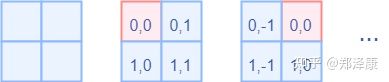
首先我们利用torch.arange和torch.meshgrid函数生成对应的坐标,这里我们以windowsize=2为例子
coords_h = torch.arange(self.window_size[0])
coords_w = torch.arange(self.window_size[1])
coords = torch.meshgrid([coords_h, coords_w]) # -> 2*(wh, ww)
"""
  (tensor([[0, 0],
           [1, 1]]),
   tensor([[0, 1],
           [0, 1]]))
"""
然后堆叠起来,展开为一个二维向量
coords = torch.stack(coords)  # 2, Wh, Ww
coords_flatten = torch.flatten(coords, 1)  # 2, Wh*Ww
"""
tensor([[0, 0, 1, 1],
        [0, 1, 0, 1]])
"""
利用广播机制,分别在第一维,第二维,插入一个维度,进行广播相减,得到 2, whww, whww的张量
relative_coords_first = coords_flatten[:, :, None]  # 2, wh*ww, 1
relative_coords_second = coords_flatten[:, None, :] # 2, 1, wh*ww
relative_coords = relative_coords_first - relative_coords_second # 最终得到 2, wh*ww, wh*ww 形状的张量
因为采取的是相减,所以得到的索引是从负数开始的,我们加上偏移量,让其从0开始。
relative_coords = relative_coords.permute(1, 2, 0).contiguous() # Wh*Ww, Wh*Ww, 2
relative_coords[:, :, 0] += self.window_size[0] - 1
relative_coords[:, :, 1] += self.window_size[1] - 1
后续我们需要将其展开成一维偏移量。而对于(1,2)和(2,1)这两个坐标。在二维上是不同的,但是通过将x,y坐标相加转换为一维偏移的时候,他的偏移量是相等的。
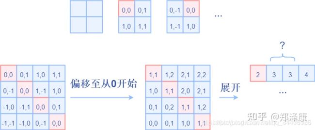
所以最后我们对其中做了个乘法操作,以进行区分
relative_coords[:, :, 0] *= 2 * self.window_size[1] - 1

然后再最后一维上进行求和,展开成一个一维坐标,并注册为一个不参与网络学习的变量
relative_position_index = relative_coords.sum(-1)  # Wh*Ww, Wh*Ww
self.register_buffer("relative_position_index", relative_position_index)
接着我们看前向代码
    def forward(self, x, mask: Optional[torch.Tensor] = None):
        """
        Args:
            x: input features with shape of (num_windows*B, Mh*Mw, C)
            mask: (0/-inf) mask with shape of (num_windows, Wh*Ww, Wh*Ww) or None
        """
        # [batch_size*num_windows, Mh*Mw, total_embed_dim]
        B_, N, C = x.shape
        # qkv(): -> [batch_size*num_windows, Mh*Mw, 3 * total_embed_dim]
        # reshape: -> [batch_size*num_windows, Mh*Mw, 3, num_heads, embed_dim_per_head]
        # permute: -> [3, batch_size*num_windows, num_heads, Mh*Mw, embed_dim_per_head]
        qkv = self.qkv(x).reshape(B_, N, 3, self.num_heads, C // self.num_heads).permute(2, 0, 3, 1, 4)
        # [batch_size*num_windows, num_heads, Mh*Mw, embed_dim_per_head]
        q, k, v = qkv.unbind(0)  # make torchscript happy (cannot use tensor as tuple)

        # transpose: -> [batch_size*num_windows, num_heads, embed_dim_per_head, Mh*Mw]
        # @: multiply -> [batch_size*num_windows, num_heads, Mh*Mw, Mh*Mw]
        q = q * self.scale
        attn = (q @ k.transpose(-2, -1))

        # relative_position_bias_table.view: [Mh*Mw*Mh*Mw,nH] -> [Mh*Mw,Mh*Mw,nH]
        relative_position_bias = self.relative_position_bias_table[self.relative_position_index.view(-1)].view(
            self.window_size[0] * self.window_size[1], self.window_size[0] * self.window_size[1], -1)
        relative_position_bias = relative_position_bias.permute(2, 0, 1).contiguous()  # [nH, Mh*Mw, Mh*Mw]
        attn = attn + relative_position_bias.unsqueeze(0)

        if mask is not None:
            # mask: [nW, Mh*Mw, Mh*Mw]
            nW = mask.shape[0]  # num_windows
            # attn.view: [batch_size, num_windows, num_heads, Mh*Mw, Mh*Mw]
            # mask.unsqueeze: [1, nW, 1, Mh*Mw, Mh*Mw]
            attn = attn.view(B_ // nW, nW, self.num_heads, N, N) + mask.unsqueeze(1).unsqueeze(0)
            attn = attn.view(-1, self.num_heads, N, N)
            attn = self.softmax(attn)
        else:
            attn = self.softmax(attn)

        attn = self.attn_drop(attn)

        # @: multiply -> [batch_size*num_windows, num_heads, Mh*Mw, embed_dim_per_head]
        # transpose: -> [batch_size*num_windows, Mh*Mw, num_heads, embed_dim_per_head]
        # reshape: -> [batch_size*num_windows, Mh*Mw, total_embed_dim]
        x = (attn @ v).transpose(1, 2).reshape(B_, N, C)
        x = self.proj(x)
        x = self.proj_drop(x)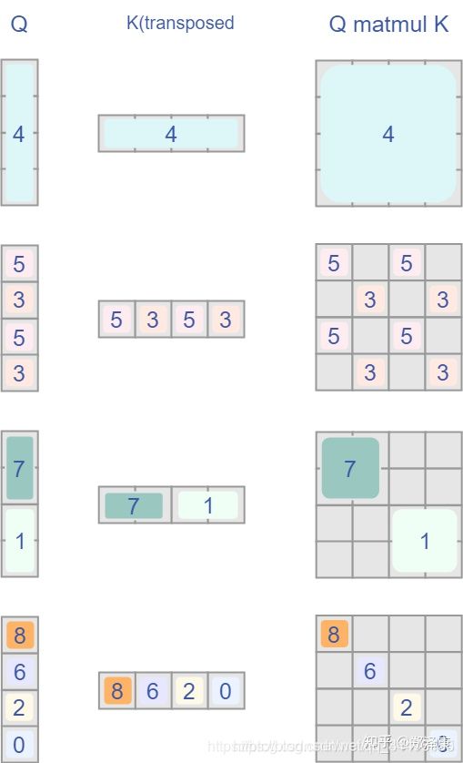
return x- 首先输入张量形状为 numWindows*B, window_size * window_size, C(后续会解释)
- 然后经过self.qkv这个全连接层后,进行reshape,调整轴的顺序,得到形状为3, numWindowsB, num_heads, window_sizewindow_size, c//num_heads,并分配给q,k,v。
- 根据公式,我们对q乘以一个scale缩放系数,然后与k(为了满足矩阵乘要求,需要将最后两个维度调换)进行相乘。得到形状为(numWindowsB, num_heads, window_sizewindow_size, window_size*window_size)的attn张量
- 之前我们针对位置编码设置了个形状为(2window_size-12window_size-1, numHeads)的可学习变量。我们用计算得到的相对编码位置索引self.relative_position_index选取,得到形状为(window_sizewindow_size, window_size*window_size, numHeads)的编码,加到attn张量上
- 暂不考虑mask的情况,剩下就是跟transformer一样的softmax,dropout,与V矩阵乘,再经过一层全连接层和dropout
3.4 Shifted Window Attention
虽然在window内部计算self-attention可能大大降低模型的复杂度,但是不同window无法进行信息交互,从而表现力欠缺。为了更好的增强模型的表现能力,引入Shifted Windows Attention。Shifted Windows是在连续的Swin Transformer blocks之间交替移动的
前面的Window Attention是在每个窗口下计算注意力的,为了更好的和其他window进行信息交互,Swin Transformer还引入了shifted window操作。
标准的Transformer架构适应于图像分类,主要采用了相对位置编码的全局自注意力机制,而全局计算的复杂度是二次的,表现为tokens的数量。这在很多视觉任务中都会带来速度损失,且在高分辨率下表现出很强的不适应性。
3.4.1 非重叠窗口的自注意力
为了高效地计算,我们采用局部窗口。这些窗口是均匀排列,且相互不重叠。假设窗口包含M×M个像素块,则 global MSA 在h×w的图像上的计算复杂度为:
![]()
![]()
这里MSA的复杂度是hw的二次方,而M^2是远小于hw的,所以它是hw的一次复杂度。
3.4.2 连续块的移位窗口划分
Shifted window partitioning in successive blocks
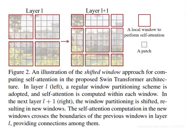
基于窗口的自注意模块缺乏跨窗口的连接,这限制了它的建模能力。为了在保持非重叠窗口计算效率的同时引入跨窗口连接,我们提出了一种 shifted window 划分方法,该方法在连续的Swin-Transformer块中交替使用两种划分配置。
如图2所示,第一个模型使用了正则窗口划分策略。从左上角开始,将8×8的像素块划分为M×M(M=4)个2×2的像素块。下一个模型的策略是shifted。对上一层划分的窗口进行移动:向左上角移动(![]() )个2×2的像素块。利用移窗划分方法,连续的Swin-Transformer块的计算公式为:
)个2×2的像素块。利用移窗划分方法,连续的Swin-Transformer块的计算公式为:

上面的公式对应了图3(b)所示的结构。
移动窗口划分策略,实现了相邻的非重叠窗口的连接,经过实验我们发现它对于图像分类、目标检测、语义分割是高效的!参考Table 4.
注意:W-MSA中的像素块特征数是一致的,但是SW-MSA它可不是一致的,这个怎么计算呢?
一般的Shifted window partition操作如下图:
- 每一个小块叫做一个patch
- 每一个深色方块框起来的叫一个local window
- 在每一个local window中计算self-attention
- 连续两个Blocks之间转换,第一个Block平分feature map,第二个Block从(⌊M/2⌋,⌊M/2⌋)像素有规律地取代前一层的windows。
windows数量变化: 例子中是2×2变成了3×3
但这种方法有一个致命的问题,就是在windows变化的过程中,有些window_size小于M × M,这就导致了需要用padding方法将其补齐使每个window大小相同,虽然解决了,但增加了计算量。
左边是没有重叠的Window Attention,而右边则是将窗口进行移位的Shift Window Attention。可以看到移位后的窗口包含了原本相邻窗口的元素。但这也引入了一个新问题,即window的个数翻倍了,由原本四个窗口变成了9个窗口。
在实际代码里,我们是通过对特征图移位,并给Attention设置mask来间接实现的。能在保持原有的window个数下,最后的计算结果等价。
window partition源码:
def window_partition(x, window_size: int):
    """
    将feature map按照window_size划分成一个个没有重叠的window
    Args:
        x: (B, H, W, C)
        window_size (int): window size(M)

    Returns:
        windows: (num_windows*B, window_size, window_size, C)
    """
    B, H, W, C = x.shape
    x = x.view(B, H // window_size, window_size, W // window_size, window_size, C)
    # permute: [B, H//Mh, Mh, W//Mw, Mw, C] -> [B, H//Mh, W//Mh, Mw, Mw, C]
    # view: [B, H//Mh, W//Mw, Mh, Mw, C] -> [B*num_windows, Mh, Mw, C]
    windows = x.permute(0, 1, 3, 2, 4, 5).contiguous().view(-1, window_size, window_size, C)
    return windows
阅读源码后发现,源码中也没有实现windows由4个变成9个的操作,而且当window_size为奇数时会报错,也不必过分纠结于此,因为实际的操作是通过下面更有效地方法计算的。
3.5 Efficient batch computation
3.5.1 shifted策略的高效batch计算
通过给Attention加mask实现,限制自注意力计算量,在子窗口中计算。
shifted操作使得像素块patches的个数⌈hM⌉×⌈wM⌉从变为(⌈h/M+1⌉×⌈w/M+1⌉)。如图2所示。且这里部分窗口的大小不是M×M。最简单的方法是直接将所有窗口padding到同样的大小。如果正则策略划分的较小,如上面的2×2,那么将增加计算量。然而我们提出了一种批量的高效计算方法:循环向左上角移动(cyclic-shifting),如下图所示:

3.6 相对位置偏置
在自注意力模块的计算中,我们引入相对位置偏置到每一个头的计算:
![]()
其中![]() 分别标识查询矩阵、键矩阵、值矩阵;d是查询矩阵或键矩阵的dimension,是窗口内的像素块个数。
分别标识查询矩阵、键矩阵、值矩阵;d是查询矩阵或键矩阵的dimension,是窗口内的像素块个数。
Note: 这里的像素块是基本像素块单元,即上文的2×2像素块,即窗口内的2×2像素块个数。
因为相对位置的范围是[−M+1,M−1],我们参数化了一个小尺寸的bias矩阵![]() ,并且我们的B是从B^中取的一个token。
,并且我们的B是从B^中取的一个token。
如表4所示,我们观察到与没有此偏差项或使用绝对位置嵌入的对应项相比有显著改进。如[19]中所述,进一步向输入中添加绝对位置嵌入会略微降低性能,因此在我们的实现中不采用这种方法。
预训练中学习到的相对位置bias矩阵也可用于初始化模型B^,以便通过双三次插值以不同的窗口大小进行微调[19,60]。
3.7 结构变体

3.8 特征图移位操作
代码里对特征图移位是通过torch.roll来实现的,下面是示意图

如果需要reverse cyclic shift的话只需把参数shifts设置为对应的正数值。
3.9 Attention Mask
我认为这是Swin Transformer的精华,通过设置合理的mask,让Shifted Window Attention在与Window Attention相同的窗口个数下,达到等价的计算结果。
首先我们对Shift Window后的每个窗口都给上index,并且做一个roll操作(window_size=2, shift_size=1)

我们希望在计算Attention的时候,让具有相同index QK进行计算,而忽略不同index QK计算结果。
最后正确的结果如下图所示
而要想在原始四个窗口下得到正确的结果,我们就必须给Attention的结果加入一个mask(如上图最右边所示)
cyclic shitf详解见文章:【Pytorch小知识】torch.roll()函数的用法及在Swin Transformer中的应用(详细易懂)
相关代码如下:
if self.shift_size > 0:
            # calculate attention mask for SW-MSA
            H, W = self.input_resolution
            img_mask = torch.zeros((1, H, W, 1))  # 1 H W 1
            h_slices = (slice(0, -self.window_size),
                        slice(-self.window_size, -self.shift_size),
                        slice(-self.shift_size, None))
            w_slices = (slice(0, -self.window_size),
                        slice(-self.window_size, -self.shift_size),
                        slice(-self.shift_size, None))
            cnt = 0
            for h in h_slices:
                for w in w_slices:
                    img_mask[:, h, w, :] = cnt
                    cnt += 1

            mask_windows = window_partition(img_mask, self.window_size)  # nW, window_size, window_size, 1
            mask_windows = mask_windows.view(-1, self.window_size * self.window_size)
            attn_mask = mask_windows.unsqueeze(1) - mask_windows.unsqueeze(2)
            attn_mask = attn_mask.masked_fill(attn_mask != 0, float(-100.0)).masked_fill(attn_mask == 0, float(0.0))
以上图的设置,我们用这段代码会得到这样的一个mask
tensor([[[[[   0.,    0.,    0.,    0.],
           [   0.,    0.,    0.,    0.],
           [   0.,    0.,    0.,    0.],
           [   0.,    0.,    0.,    0.]]],


         [[[   0., -100.,    0., -100.],
           [-100.,    0., -100.,    0.],
           [   0., -100.,    0., -100.],
           [-100.,    0., -100.,    0.]]],


         [[[   0.,    0., -100., -100.],
           [   0.,    0., -100., -100.],
           [-100., -100.,    0.,    0.],
           [-100., -100.,    0.,    0.]]],


         [[[   0., -100., -100., -100.],
           [-100.,    0., -100., -100.],
           [-100., -100.,    0., -100.],
           [-100., -100., -100.,    0.]]]]])
在之前的window attention模块的前向代码里,包含这么一段
      if mask is not None:
            nW = mask.shape[0]
            attn = attn.view(B_ // nW, nW, self.num_heads, N, N) + mask.unsqueeze(1).unsqueeze(0)
            attn = attn.view(-1, self.num_heads, N, N)
            attn = self.softmax(attn)
将mask加到attention的计算结果,并进行softmax。mask的值设置为-100,softmax后就会忽略掉对应的值
3.10 Transformer Block整体架构

两个连续的Block架构如上图所示,需要注意的是一个Stage包含的Block个数必须是偶数,因为需要交替包含一个含有Window Attention的Layer和含有Shifted Window Attention的Layer。
我们看下Block的前向代码
def forward(self, x, attn_mask):
        H, W = self.H, self.W
        B, L, C = x.shape
        assert L == H * W, "input feature has wrong size"

        shortcut = x
        x = self.norm1(x)
        x = x.view(B, H, W, C)

        # pad feature maps to multiples of window size
        # 把feature map给pad到window size的整数倍
        pad_l = pad_t = 0
        pad_r = (self.window_size - W % self.window_size) % self.window_size
        pad_b = (self.window_size - H % self.window_size) % self.window_size
        # (W_left, W_right, H_top,H_bottom, C_front, C_back)
        x = F.pad(x, (0, 0, pad_l, pad_r, pad_t, pad_b))
        _, Hp, Wp, _ = x.shape

        # cyclic shift,往右下角移动M//2
        if self.shift_size > 0:
            shifted_x = torch.roll(x, shifts=(-self.shift_size, -self.shift_size), dims=(1, 2))
        else:
            shifted_x = x
            attn_mask = None

        # partition windows
        x_windows = window_partition(shifted_x, self.window_size)  # [nW*B, Mh, Mw, C]
        x_windows = x_windows.view(-1, self.window_size * self.window_size, C)  # [nW*B, Mh*Mw, C]

        # W-MSA/SW-MSA
        attn_windows = self.attn(x_windows, mask=attn_mask)  # [nW*B, Mh*Mw, C]

        # merge windows
        attn_windows = attn_windows.view(-1, self.window_size, self.window_size, C)  # [nW*B, Mh, Mw, C]
        shifted_x = window_reverse(attn_windows, self.window_size, Hp, Wp)  # [B, H', W', C]

        # reverse cyclic shift
        if self.shift_size > 0:
            x = torch.roll(shifted_x, shifts=(self.shift_size, self.shift_size), dims=(1, 2))
        else:
            x = shifted_x

        if pad_r > 0 or pad_b > 0:
            # 把前面pad的数据移除掉
            x = x[:, :H, :W, :].contiguous()

        x = x.view(B, H * W, C)

        # FFN
        x = shortcut + self.drop_path(x)
        x = x + self.drop_path(self.mlp(self.norm2(x)))

        return x
整体流程如下:
- 先对特征图进行LayerNorm
- 通过self.shift_size决定是否需要对特征图进行shift
- 然后将特征图切成一个个窗口
- 计算Attention,通过self.attn_mask来区分Window Attention还是Shift Window Attention
- 将各个窗口合并回来
- 如果之前有做shift操作,此时进行reverse shift,把之前的shift操作恢复
- 做dropout和残差连接
- 再通过一层LayerNorm+全连接层,以及dropout和残差连接
5 实验结果

在ImageNet22K数据集上,准确率能达到惊人的86.4%。另外在检测,分割等任务上表现也很优异,感兴趣的可以翻看论文最后的实验部分。

6 存在的问题
在同尺寸通计算量的前提下,swin确实效果远好于resnet。但是有几个问题:
- 受缚于shift操作,对不同尺寸的输入要设计不同的网络,而且也要重新开始训练,这是很难接受的。
- 和Detr一样训练的时候收敛的太慢。我自己有训练了一下最小的swin-tiny版本,大概训练了一百多轮的时候也才到72~73左右。
- shift操作其实主要是为了提升感受野,可以换一种更好的方式。
7 总结
这篇文章创新点很棒,引入window这一个概念,将CNN的局部性引入,还能控制模型整体计算量。在Shift Window Attention部分,用一个mask和移位操作,很巧妙的实现计算等价。作者的代码也写得十分赏心悦目,推荐阅读!
8 模型model结构
patch_embed   PatchEmbed(
  (proj): Conv2d(3, 96, kernel_size=(4, 4), stride=(4, 4))
  (norm): LayerNorm((96,), eps=1e-05, elementwise_affine=True)
)

pos_drop   Dropout(p=0.0, inplace=False)
layers   ModuleList(
  (0): BasicLayer(
    (blocks): ModuleList(
      (0): SwinTransformerBlock(
        (norm1): LayerNorm((96,), eps=1e-05, elementwise_affine=True)
        (attn): WindowAttention(
          (qkv): Linear(in_features=96, out_features=288, bias=True)
          (attn_drop): Dropout(p=0.0, inplace=False)
          (proj): Linear(in_features=96, out_features=96, bias=True)
          (proj_drop): Dropout(p=0.0, inplace=False)
          (softmax): Softmax(dim=-1)
        )
        (drop_path): Identity()
        (norm2): LayerNorm((96,), eps=1e-05, elementwise_affine=True)
        (mlp): Mlp(
          (fc1): Linear(in_features=96, out_features=384, bias=True)
          (act): GELU()
          (drop1): Dropout(p=0.0, inplace=False)
          (fc2): Linear(in_features=384, out_features=96, bias=True)
          (drop2): Dropout(p=0.0, inplace=False)
        )
      )
      (1): SwinTransformerBlock(
        (norm1): LayerNorm((96,), eps=1e-05, elementwise_affine=True)
        (attn): WindowAttention(
          (qkv): Linear(in_features=96, out_features=288, bias=True)
          (attn_drop): Dropout(p=0.0, inplace=False)
          (proj): Linear(in_features=96, out_features=96, bias=True)
          (proj_drop): Dropout(p=0.0, inplace=False)
          (softmax): Softmax(dim=-1)
        )
        (drop_path): DropPath()
        (norm2): LayerNorm((96,), eps=1e-05, elementwise_affine=True)
        (mlp): Mlp(
          (fc1): Linear(in_features=96, out_features=384, bias=True)
          (act): GELU()
          (drop1): Dropout(p=0.0, inplace=False)
          (fc2): Linear(in_features=384, out_features=96, bias=True)
          (drop2): Dropout(p=0.0, inplace=False)
        )
      )
    )
    ************************************************
    (downsample): PatchMerging(
      (reduction): Linear(in_features=384, out_features=192, bias=False)
      (norm): LayerNorm((384,), eps=1e-05, elementwise_affine=True)
    )
  )
*********************************************************************************
  (1): BasicLayer(
    (blocks): ModuleList(
      (0): SwinTransformerBlock(
        (norm1): LayerNorm((192,), eps=1e-05, elementwise_affine=True)
        (attn): WindowAttention(
          (qkv): Linear(in_features=192, out_features=576, bias=True)
          (attn_drop): Dropout(p=0.0, inplace=False)
          (proj): Linear(in_features=192, out_features=192, bias=True)
          (proj_drop): Dropout(p=0.0, inplace=False)
          (softmax): Softmax(dim=-1)
        )
        (drop_path): DropPath()
        (norm2): LayerNorm((192,), eps=1e-05, elementwise_affine=True)
        (mlp): Mlp(
          (fc1): Linear(in_features=192, out_features=768, bias=True)
          (act): GELU()
          (drop1): Dropout(p=0.0, inplace=False)
          (fc2): Linear(in_features=768, out_features=192, bias=True)
          (drop2): Dropout(p=0.0, inplace=False)
        )
      )
      (1): SwinTransformerBlock(
        (norm1): LayerNorm((192,), eps=1e-05, elementwise_affine=True)
        (attn): WindowAttention(
          (qkv): Linear(in_features=192, out_features=576, bias=True)
          (attn_drop): Dropout(p=0.0, inplace=False)
          (proj): Linear(in_features=192, out_features=192, bias=True)
          (proj_drop): Dropout(p=0.0, inplace=False)
          (softmax): Softmax(dim=-1)
        )
        (drop_path): DropPath()
        (norm2): LayerNorm((192,), eps=1e-05, elementwise_affine=True)
        (mlp): Mlp(
          (fc1): Linear(in_features=192, out_features=768, bias=True)
          (act): GELU()
          (drop1): Dropout(p=0.0, inplace=False)
          (fc2): Linear(in_features=768, out_features=192, bias=True)
          (drop2): Dropout(p=0.0, inplace=False)
        )
      )
    )
    ************************************************
    (downsample): PatchMerging(
      (reduction): Linear(in_features=768, out_features=384, bias=False)
      (norm): LayerNorm((768,), eps=1e-05, elementwise_affine=True)
    )
  )
*********************************************************************************
  (2): BasicLayer(
    (blocks): ModuleList(
      (0): SwinTransformerBlock(
        (norm1): LayerNorm((384,), eps=1e-05, elementwise_affine=True)
        (attn): WindowAttention(
          (qkv): Linear(in_features=384, out_features=1152, bias=True)
          (attn_drop): Dropout(p=0.0, inplace=False)
          (proj): Linear(in_features=384, out_features=384, bias=True)
          (proj_drop): Dropout(p=0.0, inplace=False)
          (softmax): Softmax(dim=-1)
        )
        (drop_path): DropPath()
        (norm2): LayerNorm((384,), eps=1e-05, elementwise_affine=True)
        (mlp): Mlp(
          (fc1): Linear(in_features=384, out_features=1536, bias=True)
          (act): GELU()
          (drop1): Dropout(p=0.0, inplace=False)
          (fc2): Linear(in_features=1536, out_features=384, bias=True)
          (drop2): Dropout(p=0.0, inplace=False)
        )
      )
      ************************************************
      (1): SwinTransformerBlock(
        (norm1): LayerNorm((384,), eps=1e-05, elementwise_affine=True)
        (attn): WindowAttention(
          (qkv): Linear(in_features=384, out_features=1152, bias=True)
          (attn_drop): Dropout(p=0.0, inplace=False)
          (proj): Linear(in_features=384, out_features=384, bias=True)
          (proj_drop): Dropout(p=0.0, inplace=False)
          (softmax): Softmax(dim=-1)
        )
        (drop_path): DropPath()
        (norm2): LayerNorm((384,), eps=1e-05, elementwise_affine=True)
        (mlp): Mlp(
          (fc1): Linear(in_features=384, out_features=1536, bias=True)
          (act): GELU()
          (drop1): Dropout(p=0.0, inplace=False)
          (fc2): Linear(in_features=1536, out_features=384, bias=True)
          (drop2): Dropout(p=0.0, inplace=False)
        )
      )
      ************************************************
      (2): SwinTransformerBlock(
        (norm1): LayerNorm((384,), eps=1e-05, elementwise_affine=True)
        (attn): WindowAttention(
          (qkv): Linear(in_features=384, out_features=1152, bias=True)
          (attn_drop): Dropout(p=0.0, inplace=False)
          (proj): Linear(in_features=384, out_features=384, bias=True)
          (proj_drop): Dropout(p=0.0, inplace=False)
          (softmax): Softmax(dim=-1)
        )
        (drop_path): DropPath()
        (norm2): LayerNorm((384,), eps=1e-05, elementwise_affine=True)
        (mlp): Mlp(
          (fc1): Linear(in_features=384, out_features=1536, bias=True)
          (act): GELU()
          (drop1): Dropout(p=0.0, inplace=False)
          (fc2): Linear(in_features=1536, out_features=384, bias=True)
          (drop2): Dropout(p=0.0, inplace=False)
        )
      )
      ************************************************
      (3): SwinTransformerBlock(
        (norm1): LayerNorm((384,), eps=1e-05, elementwise_affine=True)
        (attn): WindowAttention(
          (qkv): Linear(in_features=384, out_features=1152, bias=True)
          (attn_drop): Dropout(p=0.0, inplace=False)
          (proj): Linear(in_features=384, out_features=384, bias=True)
          (proj_drop): Dropout(p=0.0, inplace=False)
          (softmax): Softmax(dim=-1)
        )
        (drop_path): DropPath()
        (norm2): LayerNorm((384,), eps=1e-05, elementwise_affine=True)
        (mlp): Mlp(
          (fc1): Linear(in_features=384, out_features=1536, bias=True)
          (act): GELU()
          (drop1): Dropout(p=0.0, inplace=False)
          (fc2): Linear(in_features=1536, out_features=384, bias=True)
          (drop2): Dropout(p=0.0, inplace=False)
        )
      )
      ************************************************
      (4): SwinTransformerBlock(
        (norm1): LayerNorm((384,), eps=1e-05, elementwise_affine=True)
        (attn): WindowAttention(
          (qkv): Linear(in_features=384, out_features=1152, bias=True)
          (attn_drop): Dropout(p=0.0, inplace=False)
          (proj): Linear(in_features=384, out_features=384, bias=True)
          (proj_drop): Dropout(p=0.0, inplace=False)
          (softmax): Softmax(dim=-1)
        )
        (drop_path): DropPath()
        (norm2): LayerNorm((384,), eps=1e-05, elementwise_affine=True)
        (mlp): Mlp(
          (fc1): Linear(in_features=384, out_features=1536, bias=True)
          (act): GELU()
          (drop1): Dropout(p=0.0, inplace=False)
          (fc2): Linear(in_features=1536, out_features=384, bias=True)
          (drop2): Dropout(p=0.0, inplace=False)
        )
      )
      ************************************************
      (5): SwinTransformerBlock(
        (norm1): LayerNorm((384,), eps=1e-05, elementwise_affine=True)
        (attn): WindowAttention(
          (qkv): Linear(in_features=384, out_features=1152, bias=True)
          (attn_drop): Dropout(p=0.0, inplace=False)
          (proj): Linear(in_features=384, out_features=384, bias=True)
          (proj_drop): Dropout(p=0.0, inplace=False)
          (softmax): Softmax(dim=-1)
        )
        (drop_path): DropPath()
        (norm2): LayerNorm((384,), eps=1e-05, elementwise_affine=True)
        (mlp): Mlp(
          (fc1): Linear(in_features=384, out_features=1536, bias=True)
          (act): GELU()
          (drop1): Dropout(p=0.0, inplace=False)
          (fc2): Linear(in_features=1536, out_features=384, bias=True)
          (drop2): Dropout(p=0.0, inplace=False)
        )
      )
    )
    (downsample): PatchMerging(
      (reduction): Linear(in_features=1536, out_features=768, bias=False)
      (norm): LayerNorm((1536,), eps=1e-05, elementwise_affine=True)
    )
  )
*********************************************************************************
  (3): BasicLayer(
    (blocks): ModuleList(
      (0): SwinTransformerBlock(
        (norm1): LayerNorm((768,), eps=1e-05, elementwise_affine=True)
        (attn): WindowAttention(
          (qkv): Linear(in_features=768, out_features=2304, bias=True)
          (attn_drop): Dropout(p=0.0, inplace=False)
          (proj): Linear(in_features=768, out_features=768, bias=True)
          (proj_drop): Dropout(p=0.0, inplace=False)
          (softmax): Softmax(dim=-1)
        )
        (drop_path): DropPath()
        (norm2): LayerNorm((768,), eps=1e-05, elementwise_affine=True)
        (mlp): Mlp(
          (fc1): Linear(in_features=768, out_features=3072, bias=True)
          (act): GELU()
          (drop1): Dropout(p=0.0, inplace=False)
          (fc2): Linear(in_features=3072, out_features=768, bias=True)
          (drop2): Dropout(p=0.0, inplace=False)
        )
      )
      ************************************************
      (1): SwinTransformerBlock(
        (norm1): LayerNorm((768,), eps=1e-05, elementwise_affine=True)
        (attn): WindowAttention(
              (qkv): Linear(in_features=768, out_features=2304, bias=True)
              (attn_drop): Dropout(p=0.0, inplace=False)
              (proj): Linear(in_features=768, out_features=768, bias=True)
              (proj_drop): Dropout(p=0.0, inplace=False)
              (softmax): Softmax(dim=-1)
                )
        (drop_path): DropPath()
        (norm2): LayerNorm((768,), eps=1e-05, elementwise_affine=True)
        (mlp): Mlp(
              (fc1): Linear(in_features=768, out_features=3072, bias=True)
              (act): GELU()
              (drop1): Dropout(p=0.0, inplace=False)
              (fc2): Linear(in_features=3072, out_features=768, bias=True)
              (drop2): Dropout(p=0.0, inplace=False)
                )
          )
        )
      )
    )

norm   LayerNorm((768,), eps=1e-05, elementwise_affine=True)
avgpool   AdaptiveAvgPool1d(output_size=1)
head   Linear(in_features=768, out_features=5, bias=True)
Backend Qt5Agg is interactive backend. Turning interactive mode on.
9 权重结构
patch_embed.proj.weight   torch.Size([96, 3, 4, 4])
patch_embed.proj.bias   torch.Size([96])
patch_embed.norm.weight   torch.Size([96])
patch_embed.norm.bias   torch.Size([96])

layers.0.blocks.0.norm1.weight   torch.Size([96])
layers.0.blocks.0.norm1.bias   torch.Size([96])
layers.0.blocks.0.attn.qkv.weight   torch.Size([288, 96])
layers.0.blocks.0.attn.qkv.bias   torch.Size([288])
layers.0.blocks.0.attn.proj.weight   torch.Size([96, 96])
layers.0.blocks.0.attn.proj.bias   torch.Size([96])
layers.0.blocks.0.norm2.weight   torch.Size([96])
layers.0.blocks.0.norm2.bias   torch.Size([96])
layers.0.blocks.0.mlp.fc1.weight   torch.Size([384, 96])
layers.0.blocks.0.mlp.fc1.bias   torch.Size([384])
layers.0.blocks.0.mlp.fc2.weight   torch.Size([96, 384])
layers.0.blocks.0.mlp.fc2.bias   torch.Size([96])
layers.0.blocks.1.norm1.weight   torch.Size([96])
layers.0.blocks.1.norm1.bias   torch.Size([96])
layers.0.blocks.1.attn.qkv.weight   torch.Size([288, 96])
layers.0.blocks.1.attn.qkv.bias   torch.Size([288])
layers.0.blocks.1.attn.proj.weight   torch.Size([96, 96])
layers.0.blocks.1.attn.proj.bias   torch.Size([96])
layers.0.blocks.1.norm2.weight   torch.Size([96])
layers.0.blocks.1.norm2.bias   torch.Size([96])
layers.0.blocks.1.mlp.fc1.weight   torch.Size([384, 96])
layers.0.blocks.1.mlp.fc1.bias   torch.Size([384])
layers.0.blocks.1.mlp.fc2.weight   torch.Size([96, 384])
layers.0.blocks.1.mlp.fc2.bias   torch.Size([96])
layers.0.downsample.norm.weight   torch.Size([384])
layers.0.downsample.norm.bias   torch.Size([384])

layers.1.blocks.0.norm1.weight   torch.Size([192])
layers.1.blocks.0.norm1.bias   torch.Size([192])
layers.1.blocks.0.attn.qkv.weight   torch.Size([576, 192])
layers.1.blocks.0.attn.qkv.bias   torch.Size([576])
layers.1.blocks.0.attn.proj.weight   torch.Size([192, 192])
layers.1.blocks.0.attn.proj.bias   torch.Size([192])
layers.1.blocks.0.norm2.weight   torch.Size([192])
layers.1.blocks.0.norm2.bias   torch.Size([192])
layers.1.blocks.0.mlp.fc1.weight   torch.Size([768, 192])
layers.1.blocks.0.mlp.fc1.bias   torch.Size([768])
layers.1.blocks.0.mlp.fc2.weight   torch.Size([192, 768])
layers.1.blocks.0.mlp.fc2.bias   torch.Size([192])
layers.1.blocks.1.norm1.weight   torch.Size([192])
layers.1.blocks.1.norm1.bias   torch.Size([192])
layers.1.blocks.1.attn.qkv.weight   torch.Size([576, 192])
layers.1.blocks.1.attn.qkv.bias   torch.Size([576])
layers.1.blocks.1.attn.proj.weight   torch.Size([192, 192])
layers.1.blocks.1.attn.proj.bias   torch.Size([192])
layers.1.blocks.1.norm2.weight   torch.Size([192])
layers.1.blocks.1.norm2.bias   torch.Size([192])
layers.1.blocks.1.mlp.fc1.weight   torch.Size([768, 192])
layers.1.blocks.1.mlp.fc1.bias   torch.Size([768])
layers.1.blocks.1.mlp.fc2.weight   torch.Size([192, 768])
layers.1.blocks.1.mlp.fc2.bias   torch.Size([192])
layers.1.downsample.norm.weight   torch.Size([768])
layers.1.downsample.norm.bias   torch.Size([768])

layers.2.blocks.0.norm1.weight   torch.Size([384])
layers.2.blocks.0.norm1.bias   torch.Size([384])
layers.2.blocks.0.attn.qkv.weight   torch.Size([1152, 384])
layers.2.blocks.0.attn.qkv.bias   torch.Size([1152])
layers.2.blocks.0.attn.proj.weight   torch.Size([384, 384])
layers.2.blocks.0.attn.proj.bias   torch.Size([384])
layers.2.blocks.0.norm2.weight   torch.Size([384])
layers.2.blocks.0.norm2.bias   torch.Size([384])
layers.2.blocks.0.mlp.fc1.weight   torch.Size([1536, 384])
layers.2.blocks.0.mlp.fc1.bias   torch.Size([1536])
layers.2.blocks.0.mlp.fc2.weight   torch.Size([384, 1536])
layers.2.blocks.0.mlp.fc2.bias   torch.Size([384])
layers.2.blocks.1.norm1.weight   torch.Size([384])
layers.2.blocks.1.norm1.bias   torch.Size([384])
layers.2.blocks.1.attn.qkv.weight   torch.Size([1152, 384])
layers.2.blocks.1.attn.qkv.bias   torch.Size([1152])
layers.2.blocks.1.attn.proj.weight   torch.Size([384, 384])
layers.2.blocks.1.attn.proj.bias   torch.Size([384])
layers.2.blocks.1.norm2.weight   torch.Size([384])
layers.2.blocks.1.norm2.bias   torch.Size([384])
layers.2.blocks.1.mlp.fc1.weight   torch.Size([1536, 384])
layers.2.blocks.1.mlp.fc1.bias   torch.Size([1536])
layers.2.blocks.1.mlp.fc2.weight   torch.Size([384, 1536])
layers.2.blocks.1.mlp.fc2.bias   torch.Size([384])
layers.2.blocks.2.norm1.weight   torch.Size([384])
layers.2.blocks.2.norm1.bias   torch.Size([384])
layers.2.blocks.2.attn.qkv.weight   torch.Size([1152, 384])
layers.2.blocks.2.attn.qkv.bias   torch.Size([1152])
layers.2.blocks.2.attn.proj.weight   torch.Size([384, 384])
layers.2.blocks.2.attn.proj.bias   torch.Size([384])
layers.2.blocks.2.norm2.weight   torch.Size([384])
layers.2.blocks.2.norm2.bias   torch.Size([384])
layers.2.blocks.2.mlp.fc1.weight   torch.Size([1536, 384])
layers.2.blocks.2.mlp.fc1.bias   torch.Size([1536])
layers.2.blocks.2.mlp.fc2.weight   torch.Size([384, 1536])
layers.2.blocks.2.mlp.fc2.bias   torch.Size([384])
layers.2.blocks.3.norm1.weight   torch.Size([384])
layers.2.blocks.3.norm1.bias   torch.Size([384])
layers.2.blocks.3.attn.qkv.weight   torch.Size([1152, 384])
layers.2.blocks.3.attn.qkv.bias   torch.Size([1152])
layers.2.blocks.3.attn.proj.weight   torch.Size([384, 384])
layers.2.blocks.3.attn.proj.bias   torch.Size([384])
layers.2.blocks.3.norm2.weight   torch.Size([384])
layers.2.blocks.3.norm2.bias   torch.Size([384])
layers.2.blocks.3.mlp.fc1.weight   torch.Size([1536, 384])
layers.2.blocks.3.mlp.fc1.bias   torch.Size([1536])
layers.2.blocks.3.mlp.fc2.weight   torch.Size([384, 1536])
layers.2.blocks.3.mlp.fc2.bias   torch.Size([384])
layers.2.blocks.4.norm1.weight   torch.Size([384])
layers.2.blocks.4.norm1.bias   torch.Size([384])
layers.2.blocks.4.attn.qkv.weight   torch.Size([1152, 384])
layers.2.blocks.4.attn.qkv.bias   torch.Size([1152])
layers.2.blocks.4.attn.proj.weight   torch.Size([384, 384])
layers.2.blocks.4.attn.proj.bias   torch.Size([384])
layers.2.blocks.4.norm2.weight   torch.Size([384])
layers.2.blocks.4.norm2.bias   torch.Size([384])
layers.2.blocks.4.mlp.fc1.weight   torch.Size([1536, 384])
layers.2.blocks.4.mlp.fc1.bias   torch.Size([1536])
layers.2.blocks.4.mlp.fc2.weight   torch.Size([384, 1536])
layers.2.blocks.4.mlp.fc2.bias   torch.Size([384])
layers.2.blocks.5.norm1.weight   torch.Size([384])
layers.2.blocks.5.norm1.bias   torch.Size([384])
layers.2.blocks.5.attn.qkv.weight   torch.Size([1152, 384])
layers.2.blocks.5.attn.qkv.bias   torch.Size([1152])
layers.2.blocks.5.attn.proj.weight   torch.Size([384, 384])
layers.2.blocks.5.attn.proj.bias   torch.Size([384])
layers.2.blocks.5.norm2.weight   torch.Size([384])
layers.2.blocks.5.norm2.bias   torch.Size([384])
layers.2.blocks.5.mlp.fc1.weight   torch.Size([1536, 384])
layers.2.blocks.5.mlp.fc1.bias   torch.Size([1536])
layers.2.blocks.5.mlp.fc2.weight   torch.Size([384, 1536])
layers.2.blocks.5.mlp.fc2.bias   torch.Size([384])
layers.2.downsample.norm.weight   torch.Size([1536])
layers.2.downsample.norm.bias   torch.Size([1536])

layers.3.blocks.0.norm1.weight   torch.Size([768])
layers.3.blocks.0.norm1.bias   torch.Size([768])
layers.3.blocks.0.attn.qkv.weight   torch.Size([2304, 768])
layers.3.blocks.0.attn.qkv.bias   torch.Size([2304])
layers.3.blocks.0.attn.proj.weight   torch.Size([768, 768])
layers.3.blocks.0.attn.proj.bias   torch.Size([768])
layers.3.blocks.0.norm2.weight   torch.Size([768])
layers.3.blocks.0.norm2.bias   torch.Size([768])
layers.3.blocks.0.mlp.fc1.weight   torch.Size([3072, 768])
layers.3.blocks.0.mlp.fc1.bias   torch.Size([3072])
layers.3.blocks.0.mlp.fc2.weight   torch.Size([768, 3072])
layers.3.blocks.0.mlp.fc2.bias   torch.Size([768])
layers.3.blocks.1.norm1.weight   torch.Size([768])
layers.3.blocks.1.norm1.bias   torch.Size([768])
layers.3.blocks.1.attn.qkv.weight   torch.Size([2304, 768])
layers.3.blocks.1.attn.qkv.bias   torch.Size([2304])
layers.3.blocks.1.attn.proj.weight   torch.Size([768, 768])
layers.3.blocks.1.attn.proj.bias   torch.Size([768])
layers.3.blocks.1.norm2.weight   torch.Size([768])
layers.3.blocks.1.norm2.bias   torch.Size([768])
layers.3.blocks.1.mlp.fc1.weight   torch.Size([3072, 768])
layers.3.blocks.1.mlp.fc1.bias   torch.Size([3072])
layers.3.blocks.1.mlp.fc2.weight   torch.Size([768, 3072])
layers.3.blocks.1.mlp.fc2.bias   torch.Size([768])

norm.weight   torch.Size([768])
norm.bias   torch.Size([768])
head.weight   torch.Size([1000, 768])
head.bias   torch.Size([1000])

layers.0.blocks.0.attn.relative_position_index   torch.Size([49, 49])
layers.0.blocks.1.attn.relative_position_index   torch.Size([49, 49])
layers.1.blocks.0.attn.relative_position_index   torch.Size([49, 49])
layers.1.blocks.1.attn.relative_position_index   torch.Size([49, 49])
layers.2.blocks.0.attn.relative_position_index   torch.Size([49, 49])
layers.2.blocks.1.attn.relative_position_index   torch.Size([49, 49])
layers.2.blocks.2.attn.relative_position_index   torch.Size([49, 49])
layers.2.blocks.3.attn.relative_position_index   torch.Size([49, 49])
layers.2.blocks.4.attn.relative_position_index   torch.Size([49, 49])
layers.2.blocks.5.attn.relative_position_index   torch.Size([49, 49])
layers.3.blocks.0.attn.relative_position_index   torch.Size([49, 49])
layers.3.blocks.1.attn.relative_position_index   torch.Size([49, 49])

layers.0.blocks.1.attn_mask   torch.Size([64, 49, 49])
layers.1.blocks.1.attn_mask   torch.Size([16, 49, 49])
layers.2.blocks.1.attn_mask   torch.Size([4, 49, 49])
layers.2.blocks.3.attn_mask   torch.Size([4, 49, 49])
layers.2.blocks.5.attn_mask   torch.Size([4, 49, 49])

layers.0.blocks.0.attn.relative_position_bias_table   torch.Size([169, 3])
layers.0.blocks.1.attn.relative_position_bias_table   torch.Size([169, 3])
layers.1.blocks.0.attn.relative_position_bias_table   torch.Size([169, 6])
layers.1.blocks.1.attn.relative_position_bias_table   torch.Size([169, 6])
layers.2.blocks.0.attn.relative_position_bias_table   torch.Size([169, 12])
layers.2.blocks.1.attn.relative_position_bias_table   torch.Size([169, 12])
layers.2.blocks.2.attn.relative_position_bias_table   torch.Size([169, 12])
layers.2.blocks.3.attn.relative_position_bias_table   torch.Size([169, 12])
layers.2.blocks.4.attn.relative_position_bias_table   torch.Size([169, 12])
layers.2.blocks.5.attn.relative_position_bias_table   torch.Size([169, 12])
layers.3.blocks.0.attn.relative_position_bias_table   torch.Size([169, 24])
layers.3.blocks.1.attn.relative_position_bias_table   torch.Size([169, 24])

layers.0.downsample.reduction.weight   torch.Size([192, 384])
layers.1.downsample.reduction.weight   torch.Size([384, 768])
layers.2.downsample.reduction.weight   torch.Size([768, 1536])

Backend Qt5Agg is interactive backend. Turning interactive mode on.
10 报错记录
Unexpected key(s) in state_dict:
layers.0.blocks.1.attn_mask
layers.1.blocks.1.attn_mask
layers.2.blocks.1.attn_mask
layers.2.blocks.3.attn_mask
layers.2.blocks.5.14:36 2022/03/04
size mismatch for head.weight: copying a param with shape torch.Size([1000, 768]) from checkpoint, the shape in current model is torch.Size([5, 768]).
size mismatch for head.bias: copying a param with shape torch.Size([1000]) from checkpoint, the shape in current model is torch.Size([5]).
11 困惑
11.1 swinT是否还需要position embedding
基本不需要,在公式中会有个相对位置编码。
11.2 SwinT论文中有提到可用于backbone,那为啥还要结合VGG16等
只是结合的VGG16的预训练参数。
11.3 SwinT的Hierarchical层级设计是如何体现的
所谓的层级设计就是指不同stage的tokens数量依次变小,为H/4×W/4、H/8×W/8、H/16×W/16、H/32×W/32,呈逐步变小的规律。
11.4 swin在哪里体现query
对于该窗口内的每一个像素(或称token,patch)在进行MSA计算时,都要先生成对应的query(q),key(k),value(v)。
12 参考链接
Swin-Transformer网络结构详解_霹雳吧啦Wz-CSDN博客_swin transformer结构文章目录0 前言1 网络整体框架2 Patch Merging详解3 W-MSA详解Ω(MSA)\Omega (MSA)Ω(MSA)模块计算量Ω(W−MSA)\Omega (W-MSA)Ω(W−MSA)模块计算量4 SW-MSA详解5 Relative Position Bias详解6 模型详细配置参数0 前言Swin Transformer是2021年微软研究院发表在ICCV上的一篇文章,并且已经获得ICCV 2021 best paper的荣誉称号。Swin Transformer网络是Tranhttps://blog.csdn.net/qq_37541097/article/details/121119988?spm=1001.2014.3001.5506
swin transformer解读_我爱那湛蓝的博客-CSDN博客_swin transformer 论文原文论文链接:Swin Transformer: Hierarchical Vision Transformer using Shifted Windows源码地址:https://github.com/microsoft/Swin-Transformer引言目前Transformer应用到图像领域主要有两大挑战:视觉实体变化大,在不同场景下视觉Transformer性能未必很好。即目标尺寸多变。不像NLP任务中token大小基本相同,目标检测中的目标尺寸不一,用单层级的模型很难有好的效果。图https://blog.csdn.net/qq_31473155/article/details/118596587