吴恩达机器学习课上lab C1_W1_Lab02_Course_Preview_Soln-checkpoint

前置

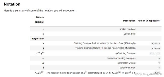
接下来将会碰到的概念

代码块1

import numpy as np#导入大名鼎鼎的numpy包
import matplotlib.pyplot as plt
plt.style.use('./deeplearning.mplstyle')

注意！
1.运行此代码需要将deeplearning.mplstyle导入至目录下

2.后面的as的意思是在导入后为了编写程序方便，给numpy起了个别名，所以在程序中直接写np指的就是numpy！

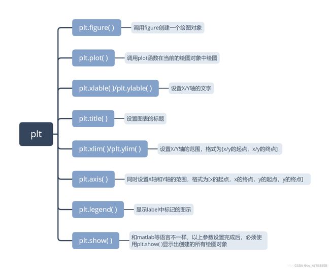
3.Matplotlib是Python的一个绘图库，是Python中最常用的可视化工具之一，可以非常方便地创建2D图表和一些基本的3D图表。
API如下

代码块2

# x_train is the input variable (size in 1000 square feet)
# y_train is the target (price in 1000s of dollars)
x_train = np.array([1.0, 2.0,4.0])
y_train = np.array([300.0, 500.0,200.0])
z_train = np.array([3000.0,50])
print(f"x_train = {x_train}")
print(f"y_train = {y_train}")
print(f"y_train = {z_train}")

输出：
x_train = [1. 2. 4.]
y_train = [300. 500. 200.]
y_train = [3000. 50.]

本课程将在打印时经常使用此处描述的python“f-string”输出格式。在生成输出时计算大括号之间的内容。

上面x,y,z都是一维数组，在后面我们会学到如何创建多维数组

代码块3

# m is the number of training examples
print(f"x_train.shape: {x_train.shape}")
m = x_train.shape[0]
print(f"Number of training examples is: {m}")

输出：
x_train.shape: (3,)
Number of training examples is: 3

注意！
Numpy数组具有.shape参数，shape函数是numpy.core.fromnumeric中的函数，它的功能是读取矩阵的长度，比如shape[0]就是读取矩阵第一维度的长度。

代码块4

m = len(x_train)
print(f"Number of training examples is: {m}")

输出：Number of training examples is: 3

这是读取矩阵长度的另一种方式，使用len（）

代码块5

i = 0 # Change this to 1 to see (x^1, y^1)

x_i = x_train[i]
y_i = y_train[i]
z_i = z_train[i]
print(f"(x^({i}), y^({i}),z^({i})) = ({x_i}, {y_i},{z_i})")

输出：(x^(0), y^(0), z^(0)) = (1.0, 300.0,3000.0)

x^(0), y^(0), z^(0)表示第一个样本的值

代码块6（绘制图像）

# Plot the data points
plt.scatter(x_train, y_train,  marker='h', c='k')
# Set the title
plt.title("aaa")
# Set the y-axis label

plt.ylabel('Price (in 1000s of dollars)')
# Set the x-axis label
plt.xlabel('Size (1000 sqft)')
plt.show()

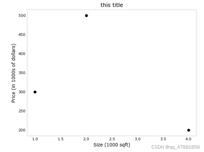
标题不能用中文暂时不知道原因，之后回来整

代码块7

#回归函数中的两个参数w和b
w = 100
b = 100
print(f"w: {w}")
print(f"b: {b}")

输出：
w: 100
b: 100

代码块8

def compute_model_output(x, w, b):
    """
    Computes the prediction of a linear model
    Args:
      x (ndarray (m,)): Data, m examples 
      w,b (scalar)    : model parameters  
    Returns
      y (ndarray (m,)): target values
    """
    m = x.shape[0]    #获取np数组长度
    f_wb = np.zeros(m)#返回来一个给定形状和类型的用0填充的数组；
    for i in range(m):
        f_wb[i] = w * x[i] + b#计算数组中的值
        
    return f_wb

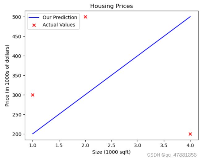
代码块9（调用compute_model_output绘制图像）

tmp_f_wb = compute_model_output(x_train, w, b,)
#绘制我们的预测模型
plt.plot(x_train, tmp_f_wb, c='b',label='Our Prediction')
#绘制数据点
plt.scatter(x_train, y_train, marker='x', c='r',label='Actual Values')
#标题
plt.title("Housing Prices")
#设置Y轴的标签
plt.ylabel('Price (in 1000s of dollars)')
#设置X轴的标签
plt.xlabel('Size (1000 sqft)')
plt.legend()
plt.show()

输出

代码块10（使用我们的模型做预测）

w = 200                         
b = 100    
x_i = 1.2
cost_1200sqft = w * x_i + b    

print(f"${cost_1200sqft:.0f} thousand dollars")

输出：
$340 thousand dollars

总结

1.学会了回归（regression）模型的建立；
2.学会了使用python进行基本图像的绘制；