python机器学习笔记（二）：分类算法——感知机

• 分类机器学习算法：

  • 感知器perceptron
  • 自适应性神经元adaptive linear neuron

  内容：

  • 使用pandas、NumPy和matplotlib读取、处理和可视化数据
  • 使用python实现线性分类算法

感知器算法实现

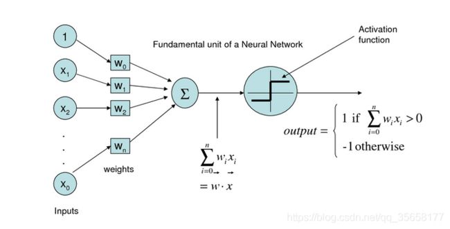
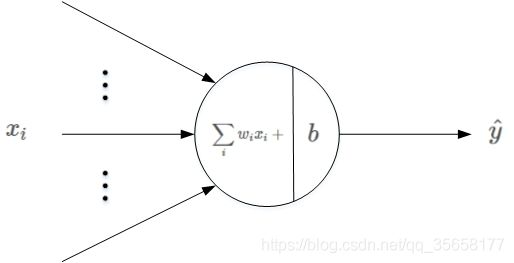
• 感知器模型
  

• 感知器学习规则
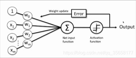  输入训练样本X和初始权重向量W，将其进行向量的点乘，然后将点乘求和的结果作用于激活函数sign（），得到预测输出O，根据预测输出值和目标值之间的差距error，来调整初始化权重向量W。如此反复，直到W调整到合适的结果为止。

• 算法的原始形式
  

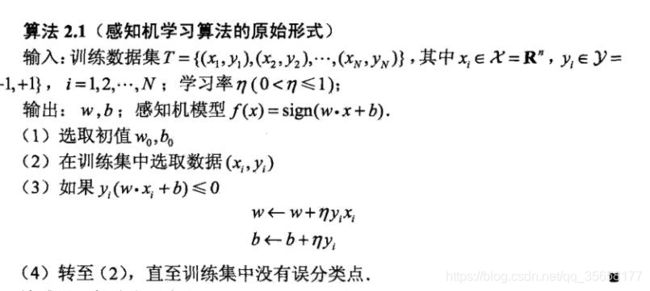
参考：https://blog.csdn.net/red_stone1/article/details/80491895

-算法：

#感知器算法
import numpy as np
class Perceptron(object):
    '''
    Perceptron classifier(感知器分类器)
    Parameters(参数)
    ---------------------
    eta:float 学习率
        Learning rate(between 0.0 and 1.0)
    n_iter:int 权重向量的训练次数
        Passes over training dataset 
    
    Attributes(属性)
    ---------------------
    w_: 1d_array 一维权重向量
        Weights after fitting
    errors_: list 记录神经元判断错误的次数
        Number of misclassifications in every epoch
     
    '''
    #初始化对象
    def __init__(self,eta=0.01,n_iter=10):  #eta:学习率；n_iter:在训练集上进行迭代的次数
        self.eta = eta
        self.n_iter = n_iter
    
    #训练模型
    def fit(self,X,y):
        '''
        fit training data.(拟合训练数据)
        
        Parameters(参数)
        -------------------
        X: {array-like},shape = [n_samples, n_features]
           Trainig vectors,where n_samples is the number of samples and n_features is the number of features
        y: arrat-like, shape = [n_samples]
           Target values
        X为n行m列的训练样本矩阵(n个样本，m个特征值)；y为目标矩阵n行1列
        
        Returns
        ---------------
        self : object
        '''
        ##对于那些并非在初始化对象时创建但是又被对象中其他方法调用的属性，可以在后面添加一个下划线，例如self.w_
        self.w_ = np.zeros(1 + X.shape[1])   #self.w_为权值，初始化为0向量(一维矩阵) ;shape属性返回维数，shape[0]返回行数，shape[1]返回列数
        self.errors_ =[]                     #self.error_为误差
        for _ in range(self.n_iter):      #下划线表示临时变量, 仅用一次,后面无需再用到
            errors = 0
            for xi, target in zip(X,y):     #zip()函数见下解释;xi,target为一条样本的特征值(训练数)及目标值
                update = self.eta*(target - self.predict(xi))  #计算预测与实际值之间的误差在乘以学习率
                self.w_[1:] += update * xi   #更新后的权重
                self.w_[0] += update        #偏移常数？
                errors += int(update!=0.0)   #记录每次迭代误差的总值
            self.errors_.append(errors)
        return self
    
    def net_input(self, X):
        return np.dot(X, self.w_[1:]) + self.w_[0]  #两个一维数组的dot，进行内积，返回一个数
    
    def predict(self, X):
        return np.where(self.net_input(X) >= 0.0, 1, -1)   #np.where(condition, x, y)：满足条件(condition)，输出x，不满足输出y。

• zip函数

zip() 函数用于将可迭代的对象作为参数，将对象中对应的元素打包成一个个元组，然后返回由这些元组组成的对象，这样做的好处是节约了不少的内存。我们可以使用 list() 转换来输出列表。
如果各个迭代器的元素个数不一致，则返回列表长度与最短的对象相同，利用 * 号操作符，可以将元组解压为列表

a = [1,2,3]
b = [4,5,6]
c = [4,5,6,7,8]
zip1 = zip(a,b)
print(zip1)
print(list(zip1))
zip2 = zip(a,c)
print(zip2)
print(list(zip2))

输出

<zip object at 0x000001AA820DDC08>
[(1, 4), (2, 5), (3, 6)]
<zip object at 0x000001AA820E6608>
[(1, 4), (2, 5), (3, 6)]

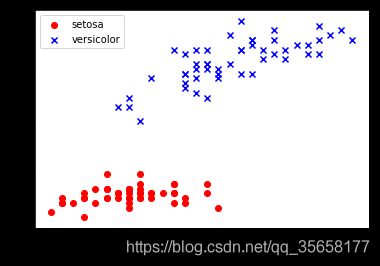
• 基于鸢尾花数据集训练感知器模型—数据可视化
• 从中提取100个类标，其中分别包含50个山鸢尾类标和50个变色鸢尾类标，并将这些类标用两个整数值来表示，1代表变色鸢尾，-1代表山鸢尾，赋值给y;
• 提取这100个训练样本的第一个特征值列（萼片长度）和第三个特征列（花瓣长度），并赋值给属性矩阵X

y = df.iloc[0:100, 4].values
y = np.where(y == 'Iris-setosa', -1, 1)
X = df.iloc[0:100, [0, 2]].values
plt.scatter(X[:50, 0], X[:50, 1], color='red', marker='o', label='setosa')
plt.scatter(X[50:100, 0], X[50:100, 1], color='blue', marker='x', label='versicolor')
plt.xlabel('petal length')
plt.ylabel('sepal length')
plt.legend(loc='upper left')
plt.show()
print(y)
print(X)

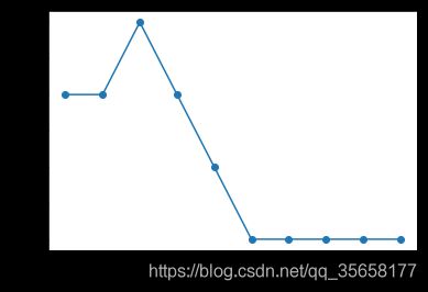
- 基于鸢尾花数据集训练感知器模型—训练感知器

ppn = Perceptron(eta = 0.1, n_iter=10)
ppn.fit(X,y)
plt.plot(range(1, len(ppn.errors_) + 1), ppn.errors_, marker = 'o')   #绘制每次迭代的错误分类数量的折线图
plt.xlabel('Epochs')
plt.ylabel('Number of misclassifications')
plt.show()

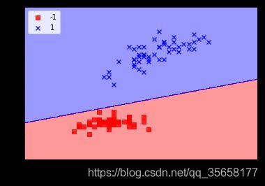
• 二维数据集决策边界的可视化

from matplotlib.colors import ListedColormap

def plot_decision_regions(X, y, classifier, resolution=0.02):
    
    #setup marker genterator and color map
    markers = ('s', 'x', 'o', '^', 'v')
    colors = ('red', 'blue', 'lightgreen', 'gray', 'cyan')
    cmap = ListedColormap(colors[:len(np.unique(y))])
    
    #plot the decision surface
    x1_min, x1_max = X[:, 0].min() - 1, X[:, 0].max() + 1
    x2_min, x2_max = X[:, 1].min() - 1, X[:, 1].max() + 1
    xx1, xx2 = np.meshgrid(np.arange(x1_min, x1_max, resolution),
                          np.arange(x2_min, x2_max, resolution))
    Z = classifier.predict(np.array([xx1.ravel(), xx2.ravel()]).T)
    Z = Z.reshape(xx1.shape)
    plt.contourf(xx1, xx2, Z, alpha=0.4, cmap=cmap)
    plt.xlim(xx1.min(), xx1.max())
    plt.ylim(xx2.min(), xx2.max())
    
    #plot class samples
    for idx, cl in enumerate(np.unique(y)):
        plt.scatter(x=X[y == cl, 0],y=X[y == cl, 1],
                   alpha=0.8, c=cmap(idx),
                   marker=markers[idx], label=cl)

plot_decision_regions(X, y, classifier=ppn)
plt.xlabel('sepal length [cm]')
plt.ylabel('petal length [cm]')
plt.legend(loc='upper left')
plt.show()

输出：