SGM and SGBM
Intro:
Wikipedia https://en.wikipedia.org/wiki/Semi-global_matching
SGM Paper:
Accurate and efficient stereo processing by semi-global matching and mutual information | IEEE Conference Publication | IEEE Xplore![]() https://ieeexplore.ieee.org/document/1467526
https://ieeexplore.ieee.org/document/1467526
https://core.ac.uk/download/pdf/11134866.pdfStereo Processing by Semiglobal Matching and Mutual Information | IEEE Journals & Magazine | IEEE Xplore![]() https://ieeexplore.ieee.org/document/4359315
https://ieeexplore.ieee.org/document/4359315
Semi-Global Matching, SGM
From Wikipedia, the free encyclopedia
Semi-global matching (SGM) is a computer vision algorithm for the estimation of a dense disparity map from a rectified stereo image pair, introduced in 2005 by Heiko Hirschmüller while working at the German Aerospace Center.[1] Given its predictable run time, its favourable trade-off between quality of the results and computing time, and its suitability for fast parallel implementation in ASIC or FPGA, it has encountered wide adoption in real-time stereo vision applications such as robotics and advanced driver assistance systems.[2][3]
Semi-Global Block Matching, SGBM
OpenCV SGBM Summary
Detailed Description
The class implements the modified H. Hirschmuller algorithm [112] that differs from the original one as follows:
- By default, the algorithm is single-pass, which means that you consider only 5 directions instead of 8. Set mode=StereoSGBM::MODE_HH in createStereoSGBM to run the full variant of the algorithm but beware that it may consume a lot of memory.
- The algorithm matches blocks, not individual pixels. Though, setting blockSize=1 reduces the blocks to single pixels.
- Mutual information cost function is not implemented. Instead, a simpler Birchfield-Tomasi sub-pixel metric from [23] is used. Though, the color images are supported as well.
- Some pre- and post- processing steps from K. Konolige algorithm StereoBM are included, for example: pre-filtering (StereoBM::PREFILTER_XSOBEL type) and post-filtering (uniqueness check, quadratic interpolation and speckle filtering).
Note
- (Python) An example illustrating the use of the StereoSGBM matching algorithm can be found at opencv_source_code/samples/python/stereo_match.py
source code: https://github.com/opencv/opencv/blob/4.x/modules/calib3d/src/stereosgbm.cpp
OpenCV源代码分析——SGBM - 知乎
立体匹配算法SGBM_殇沐的博客-CSDN博客_立体匹配算法sgbm
SGBM Breakdown
立体匹配算法推理笔记(一) - 知乎![]() https://zhuanlan.zhihu.com/p/139458878
https://zhuanlan.zhihu.com/p/139458878
the following two papers, as their names suggest, provide overviews for the various cv algorithms and strategies.
paper:https://downloads.hindawi.com/journals/js/2016/8742920.pdf
A taxonomy and evaluation of dense two-frame stereo correspondence algorithms | IEEE Conference Publication | IEEE Xplore
立体匹配算法推理笔记 - SGBM算法(一) - 知乎![]() https://zhuanlan.zhihu.com/p/139460011
https://zhuanlan.zhihu.com/p/139460011
the cost calculation (BT) is in Depth Discontinuities by Pixel-to-Pixel Stereo by
STAN BIRCHFIELD AND CARLO TOMASI section 3
立体匹配算法推理笔记 - SGBM算法(二) - 知乎![]() https://zhuanlan.zhihu.com/p/139461526
https://zhuanlan.zhihu.com/p/139461526
立体匹配算法推理笔记 - CBCA - 知乎
On building an accurate stereo matching system on graphics hardware | IEEE Conference Publication | IEEE Xplore
SGBM Performance
The KITTI Vision Benchmark Suite
Disparity Map Quality Measure
https://www.mdpi.com/2079-9292/9/10/1625/pdf
figure 1 of example ground truth (best disparity map) from the paper above can be summed up in short:
1. details in near-field ==> clear edges
2. gradual transition to far-field when possible
3. smooth bounded regions ==> ignore noise from texture ==> detailess far-field
4. sharply shaded regions can be ignored ==> better than introduced as errors
Application Example
dataset besides KITTI:
DrivingStereo | A Large-Scale Dataset for Stereo Matching in Autonomous Driving Scenarios
OpenCV
API
OpenCV: cv::StereoSGBM Class Reference
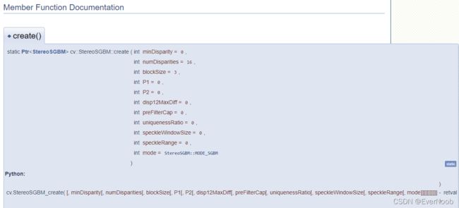
Creates StereoSGBM object.
Parameters
| minDisparity | Minimum possible disparity value. Normally, it is zero but sometimes rectification algorithms can shift images, so this parameter needs to be adjusted accordingly. |
| numDisparities | Maximum disparity minus minimum disparity. The value is always greater than zero. In the current implementation, this parameter must be divisible by 16. |
| blockSize | Matched block size. It must be an odd number >=1 . Normally, it should be somewhere in the 3..11 range. |
| P1 | The first parameter controlling the disparity smoothness. See below. |
| P2 | The second parameter controlling the disparity smoothness. The larger the values are, the smoother the disparity is. P1 is the penalty on the disparity change by plus or minus 1 between neighbor pixels. P2 is the penalty on the disparity change by more than 1 between neighbor pixels. The algorithm requires P2 > P1 . See stereo_match.cpp sample where some reasonably good P1 and P2 values are shown (like 8*number_of_image_channels*blockSize*blockSize and 32*number_of_image_channels*blockSize*blockSize , respectively). |
| disp12MaxDiff | Maximum allowed difference (in integer pixel units) in the left-right disparity check. Set it to a non-positive value to disable the check. |
| preFilterCap | Truncation value for the prefiltered image pixels. The algorithm first computes x-derivative at each pixel and clips its value by [-preFilterCap, preFilterCap] interval. The result values are passed to the Birchfield-Tomasi pixel cost function. |
| uniquenessRatio | Margin in percentage by which the best (minimum) computed cost function value should "win" the second best value to consider the found match correct. Normally, a value within the 5-15 range is good enough. |
| speckleWindowSize | Maximum size of smooth disparity regions to consider their noise speckles and invalidate. Set it to 0 to disable speckle filtering. Otherwise, set it somewhere in the 50-200 range. |
| speckleRange | Maximum disparity variation within each connected component. If you do speckle filtering, set the parameter to a positive value, it will be implicitly multiplied by 16. Normally, 1 or 2 is good enough. |
| mode | Set it to StereoSGBM::MODE_HH to run the full-scale two-pass dynamic programming algorithm. It will consume O(W*H*numDisparities) bytes, which is large for 640x480 stereo and huge for HD-size pictures. By default, it is set to false . |
The first constructor initializes StereoSGBM with all the default parameters. So, you only have to set StereoSGBM::numDisparities at minimum. The second constructor enables you to set each parameter to a custom value.
Base Version Example
opencv双目测距(BM 与SGBM匹配)_xiao__run的博客-CSDN博客_sgbm测距
KITTI下使用SGBM立体匹配算法获得深度图_逆水独流的博客-CSDN博客_kitti获取深度图
CUDA Variant
https://github.com/jasonlinuxzhang/sgbm_cuda
OpenCV: cv::cuda::StereoSGM Class Reference
MATLAB
Stereo Disparity Using Semi-Global Block Matching- MATLAB & Simulink- MathWorks 中国
SGM Parallelization
SGBM is an OpenCV variant of SGM, best optimized for CPUs; Direct attempts to optimize SGM for device massive parallelism could yield much better results.
SGM on GPU
GitHub - WanchaoYao/SGM: CPU & GPU Implementation of SGM(semi-global matching)
GitHub - dhernandez0/sgm: Semi-Global Matching on the GPU
GPU optimization of the SGM stereo algorithm | IEEE Conference Publication | IEEE Xplore
OpenCV SIMD
聊聊OpenCV的SIMD机制 - 知乎
opencv api: OpenCV: opencv2/core/hal/intrin.hpp File Reference
GPU vs. SIMD
Sensors | Free Full-Text | ReS2tAC—UAV-Borne Real-Time SGM Stereo Optimized for Embedded ARM and CUDA Devices
Related Concepts
1. Epipolar Geometry and Disparity
https://blog.csdn.net/maxzcl/article/details/122634503
2. Viterbi Algorithm
https://en.wikipedia.org/wiki/Viterbi_algorithm
From Wikipedia, the free encyclopedia
The Viterbi algorithm is a dynamic programming algorithm for obtaining the maximum a posteriori probability estimate of the most likely sequence of hidden states—called the Viterbi path—that results in a sequence of observed events, especially in the context of Markov information sources and hidden Markov models (HMM).
The algorithm has found universal application in decoding the convolutional codes used in both CDMA and GSM digital cellular, dial-up modems, satellite, deep-space communications, and 802.11 wireless LANs. It is now also commonly used in speech recognition, speech synthesis, diarization,[1] keyword spotting, computational linguistics, and bioinformatics. For example, in speech-to-text (speech recognition), the acoustic signal is treated as the observed sequence of events, and a string of text is considered to be the "hidden cause" of the acoustic signal. The Viterbi algorithm finds the most likely string of text given the acoustic signal.
3. Optical Flow
https://en.wikipedia.org/wiki/Optical_flow
Optical flow or optic flow is the pattern of apparent motion of objects, surfaces, and edges in a visual scene caused by the relative motion between an observer and a scene.[1][2] Optical flow can also be defined as the distribution of apparent velocities of movement of brightness pattern in an image.[3] The concept of optical flow was introduced by the American psychologist James J. Gibson in the 1940s to describe the visual stimulus provided to animals moving through the world.[4] Gibson stressed the importance of optic flow for affordance perception, the ability to discern possibilities for action within the environment. Followers of Gibson and his ecological approach to psychology have further demonstrated the role of the optical flow stimulus for the perception of movement by the observer in the world; perception of the shape, distance and movement of objects in the world; and the control of locomotion.[5]
The term optical flow is also used by roboticists, encompassing related techniques from image processing and control of navigation including motion detection, object segmentation, time-to-contact information, focus of expansion calculations, luminance, motion compensated encoding, and stereo disparity measurement.[6][7]
The optic flow experienced by a rotating observer. The direction and magnitude of optic flow at each location is represented by the direction and length of each arrow.
Optical flow is defined as the apparent motion of individual pixels on the image plane. It often serves as a good approximation of the true physical motion projected onto the image plane.
4. Hamming Distance
https://en.wikipedia.org/wiki/Hamming_distance
In information theory, the Hamming distance between two strings of equal length is the number of positions at which the corresponding symbols are different. In other words, it measures the minimum number of substitutions required to change one string into the other, or the minimum number of errors that could have transformed one string into the other. In a more general context, the Hamming distance is one of several string metrics for measuring the edit distance between two sequences. It is named after the American mathematician Richard Hamming.
5. Speckle
from python 3.x - What is speckle in stereo BM and SGBM algorithm implemented in OpenCV - Stack Overflow
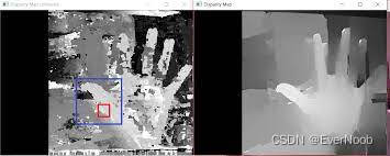
"block-based matching has problems near the boundaries of objects because the matching window catches the foreground on one side and the background on the other side. This results in a local region of large and small disparities that we call speckle. To prevent these borderline matches, we can set a speckle detector over a speckle window (ranging in size from 5-by-5 up to 21 by-21) by setting speckleWindowSize, which has a default setting of 9 for a 9-by-9 window. Within the speckle window, as long as the minimum and maximum detected disparities are within speckleRange, the match is allowed (the default range is set to 4)". ==> else the pixel (at the center of the window) is painted off by some default background value, see Cv2.FilterSpeckles Method
While using any of provided disparity algorithms it's likely to have better results if post filtering is applied. Typical problem zones of disparity maps from stereo images are object edges, shaded areas, textured regions comes from how disparity map is counted. You may check this tutorial where one type of post filtering is applied to BM disparity algorithm.
"Learning OpenCV" is a great book and your cite from it gives a clear answer to your question.
The is results in a local region of large and small disparities that we call speckle.
I took an image from the question at answers.opencv.org.
Speckle is a region with huge variance between counted disparities which should be considered as a noise (and filtered). And speckles are likely to come in problem areas.
The reason for manual setup of speckle-related parameters of algorithm is that this parameters will very between different scenes and setups. So there is not a single optimal choice of
speckleWindowSizeandspeckleRangeto fit any developer's requirements. You may work with large objects close to camera (like on the image) or with small objects far from camera and close to background (cars on bird-view road scene) etc. So you should set parameters which suit your particular camera setup (or provide your user with interface to adjust them if camera setups may vary). Consider areas around fingers and inside a palm. There are speckles (especially area inside a palm). The difference in disparity is noise in this case and should be filtered. Choosing very bigspeckleWindowSize(blue rectangle) will lead to loss of small but important details like fingers. It maybe better to choose smallerspeckleWindowSize(red rectangle) and biggerspeckleRangesince disparity variation seems to be big.
6. (Intel) Integrated Performance Primitives, IPP
Intel® IPP - Open Source Computer Vision Library (OpenCV) FAQ
http://experienceopencv.blogspot.com/2011/07/speed-up-with-intel-integrated.html

