机器学习 二分类分类阈值_分类指标和阈值介绍

机器学习 二分类分类阈值

分类评估 (Classification Evaluation)

The metric we use to evaluate our classifier depends on the nature of the problem we want to solve and the potential consequences of prediction error. Let’s examine a very common example of cancer diagnosis (ie. classified as having cancer or not having cancer). We want our model to predict as many actual/true cancer diagnoses as possible but we also know that it is statistically impossible to correctly identify all true cancer diagnoses. Our model will eventually classify/predict someone to have cancer when they actually don’t have cancer (false positive) and predict someone not to have cancer when they actually have cancer (false negative). The question we have to ask ourselves is “What is worse? Predicting someone to have cancer when they actually don’t or predicting someone not to have cancer when they do?”. The answer in this example is obvious as the consequences of telling someone they don’t have cancer when they do far outweigh the former. Let’s keep this example in mind but let’s review the commonly used classification performance metrics.

我们用来评估分类器的指标取决于我们要解决的问题的性质以及预测误差的潜在后果。 让我们检查一个非常常见的癌症诊断示例(即，分类为患有癌症或未患有癌症)。 我们希望我们的模型能够预测尽可能多的实际/真实癌症诊断，但我们也知道，从统计上讲不可能正确识别所有真实的癌症诊断。 我们的模型最终将分类/预测某人实际上没有癌症时(假阳性)患有癌症，并预测某人实际上没有癌症时(假阴性)患有癌症。 我们必须问自己的问题是：“更糟的是什么？ 预测某人实际上没有癌症，还是预测某人没有癌症？”。 这个例子的答案是显而易见的，因为告诉某人没有癌症的后果要远远超过前者。 让我们牢记这个示例，但让我们回顾一下常用的分类性能指标。

分类效果指标 (Classification Performance Metrics)

混淆矩阵 (Confusion Matrix)

A confusion matrix summarizes are the model’s predictions. It gives us the number of correct predictions (True Positives and True Negatives) and the number of incorrect predictions (False Positives and False Negatives). In our cancer example, if our model predicted someone to have cancer and the person has cancer that’s a true positive. When our model predicted someone not to have cancer and that person does not have cancer that’s a true negative. When our model predicted someone to have cancer but that person does not have cancer that’s a false positive (ie. the model falsely predicted a positive cancer diagnosis). Finally, when our model predicted someone not to have cancer but they do that’s a false negative (ie. the model falsely predicted a negative cancer diagnosis).

混淆矩阵总结的是模型的预测。 它为我们提供了正确预测的数量(真肯定和否定)和不正确预测的数量(假肯定和否定)。 在我们的癌症示例中，如果我们的模型预测某人患有癌症并且该人患有癌症，那将是真正的阳性。 当我们的模型预测某人没有癌症，而该人没有癌症时，这是真正的负面结果。 当我们的模型预测某人患有癌症，但该人没有癌症时，即为假阳性(即该模型错误地预测为阳性癌症诊断)。 最终，当我们的模型预测某人没有癌症，但是他们这样做时，那就是假阴性(即模型错误地预测出癌症诊断为阴性)。

Much of the remaining performance metrics are derived from the confusion matrix therefore, it is imperative you have a good understand.

其余大部分性能指标均来自混淆矩阵，因此，您必须有一个很好的了解。

准确性 (Accuracy)

In simplest terms, accuracy details how often our model is correct. In other words, is the number of correct predictions (TP, TF) divided by the total number of predictions. Accuracy is typically the first metric but it can be very misleading if not considered carefully. For example, let’s consider an imbalanced dataset that was used to train our model. We have 1000 non-cancer diagnoses and 10 cancer diagnoses. A model was able to correctly predict 900 of the non-cancer diagnoses and 1 of the cancer diagnoses would have an accuracy of 0.89% ((900+1)/1010=0.89).

用最简单的术语来说，准确性详细说明了我们的模型正确的频率。 换句话说，是正确预测(TP，TF)的数量除以预测的总数。 精度通常是第一个度量标准，但是如果不仔细考虑的话，可能会产生很大的误导。 例如，让我们考虑用于训练模型的不平衡数据集。 我们有1000个非癌症诊断和10个癌症诊断。 一个模型能够正确预测900项非癌症诊断，其中1项癌症诊断的准确性为0.89％((900 + 1)/1010=0.89)。

(TP+TN)/(TP+FP+FN+TN)

(TP + TN)/(TP + FP + FN + TN)

精度(也称为特异性) (Precision (also called Specificity))

Precision tells us what percentage of the predicted positive class was correct. In other words, what percentage of predicted cancer diagnoses actually had cancer. Precision cares only that our model accurately predicted the positive class. I like to think of Precision as a measure of how “picky” or how “sure” a model is that it’s correctly predicting positive cancer diagnoses. A different example might be related to a zombie apocalypse. Even allowing one infected zombie into your camp will cause everyone to get infected. A model that has high precision would make sure that those people you let into your camp are healthy. However, the model would also have a high false-negative count (ie. healthy people who are considered infected). High precision relates to low FP rates. Preferred when the consequences of false positives are high.

精确度告诉我们预测的阳性类别中正确的百分比。 换句话说，预测癌症诊断出的癌症实际百分比是多少。 精度只关心我们的模型准确地预测了阳性类别。 我喜欢将Precision视为衡量模型正确预测癌症诊断的准确程度的一种方法。 一个不同的例子可能与僵尸启示录有关。 即使允许一个被感染的僵尸进入您的营地，也会导致每个人都被感染。 具有高精度的模型可以确保您放进营地的那些人健康。 但是，该模型还将具有较高的假阴性计数(即，被认为感染了健康的人)。 高精度与低FP率有关。 当误报的后果很高时，首选。

TP/(TP+FP)

TP /(TP + FP)

召回(也称为灵敏度) (Recall (also called Sensitivity))

Recall is the percentage of actual positives our model predicted to be positive. What percentage of people diagnosed with cancer (by a doctor) our model predicted to have cancer. Recall cares less about accurately predicting positive cases but making sure we have captured all the positive cases since the consequences of classifying someone not to have cancer when they do are much graver. We want our model to have high recall to classify as many actual cancer diagnoses as having cancer. Unfortunately, this means that the model will also classify a larger number of individuals who do not have cancer as having cancer (ie. false positives). High recall relates to low FN rates. Preferred when the consequences of false negatives are high.

回忆是我们的模型预测为阳性的实际阳性百分比。 我们的模型预测(被医生)诊断出患有癌症的人数占癌症的百分比。 回想起来不太在乎准确地预测阳性病例，而是要确保我们捕获了所有阳性病例，因为将某人分类为没有患癌症的后果要严重得多。 我们希望我们的模型具有较高的召回率，以便将与癌症一样多的实际癌症诊断分类。 不幸的是，这意味着该模型还将把没有癌症的大量个体分类为患有癌症(即假阳性)。 高召回率与低FN率有关。 当假阴性的后果很高时，首选。

TP/(TP+FN)

TP /(TP + FN)

F1分数 (F1 Score)

It is mathematically impossible to have both high precision and high recall and this is where the F1-score comes in handy. F1-score is the harmonic average of precision and recall. If you’re trying to produce a model that balances precision and recall, F1-score is a great option. F1-score is also a good option when you have an imbalanced dataset. A good F1-score means you have low FP and low FN.

从数学上讲，不可能兼具高精度和高召回率，这就是F1得分派上用场的地方。 F1分数是精度和召回率的谐波平均值。 如果您要生成平衡精度和召回率的模型，则F1分数是一个不错的选择。 当数据集不平衡时，F1分数也是一个不错的选择。 出色的F1得分意味着您的FP和FN较低。

2*(Recall * Precision) / (Recall + Precision)

2 *(调用*精度)/(调用+精度)

ROC曲线/ AUC分数 (ROC Curve/AUC Score)

The receiver operating characteristics curve (ROC) plots the true positive rate against the false-positive rate at any probability threshold. The threshold is the specified cut off for an observation to be classified as either 0 (no cancer) or 1 (has cancer).

接收器工作特性曲线(ROC)在任何概率阈值下绘制真实的阳性率相对于假阳性率。 阈值是将观察值分类为0(无癌)或1(有癌)的指定截止值。

That was a mouthful……..

那真是令人mouth目结舌……..

This will help us better understand what is a threshold, how we can adjust the model’s prediction by changing the threshold, and how a ROC curve is created. This example will also bring in the concepts of TP, TN, FN, and FP you learned above.

这将帮助我们更好地理解什么是阈值，如何通过更改阈值来调整模型的预测以及如何创建ROC曲线。 此示例还将引入您在上面学到的TP，TN，FN和FP的概念。

Follow along all this will make sense, I promise :)

我保证，遵循所有这些都是有意义的：)

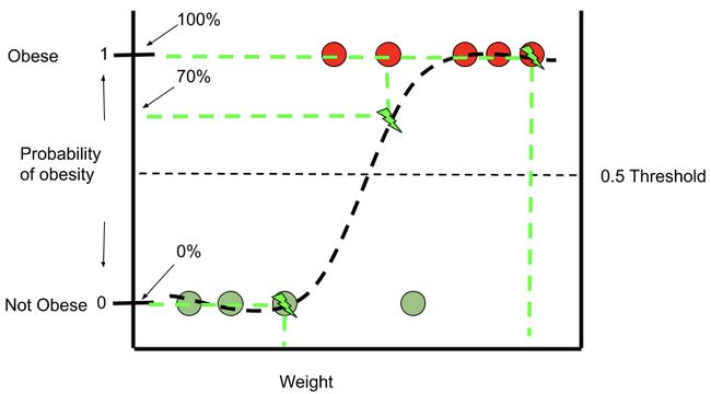
Logistic regression is a binary classifier and in the example above, we are trying to correctly predict obesity based on only one feature/predictor, weight. We have a dataset of 9 observations, where 4 (green) observations are not obese and 5 (red) are obese. Based on the sigmoid function (the curvy line) produced by the log regression the first 3 green non-obese observations have a 0% chance of being predicted as obese based on their weight. The last 3 red obese observations also have a 100% probability of being predicted as obese. The second red obese observation has a ~70% chance of being predicted as obese.

Logistic回归是一种二元分类器，在上面的示例中，我们尝试仅基于一个特征/预测因子(体重)正确预测肥胖。 我们有9个观测值的数据集，其中4个(绿色)观测值不是肥胖的，而5个(红色)观测值是肥胖的。 根据对数回归产生的S形函数(曲线)，前3个绿色非肥胖观察值的体重预测为肥胖的机率为0％。 最后3次红色肥胖的观察也有100％的概率被预测为肥胖。 第二个红色肥胖观察者有约70％的机会被预测为肥胖。

However, the 4th green non-obese observation has a ~85% chance of being predicted as obese based on its weight (must be very muscular), but we know that’s the wrong prediction. Furthermore, the first obese observation has a ~15% chance of being obese which once again the wrong prediction. Keep in mind the threshold is 0.5, therefore, any data point which falls at 51% probability of being obese will be classified as obese and any data point which falls below 50% will be classified as non-obese.

但是，第四次绿色非肥胖观察有大约85％的机会根据其体重被预测为肥胖(必须非常肌肉发达)，但我们知道这是错误的预测。 此外，首次肥胖的观察者有约15％的机会变得肥胖，这又是错误的预测。 请记住，该阈值为0.5，因此，任何肥胖率低于51％的数据点都将被归类为肥胖，而低于50％的数据点将被归类为非肥胖。

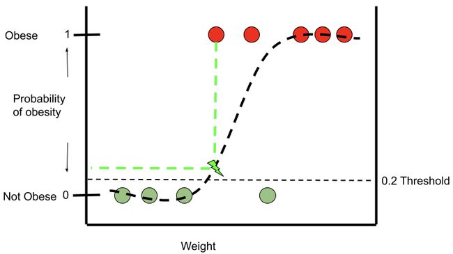
Let’s assume the consequences of incorrectly predicting someone not to be obese when they actually are obese are significant. In other words, we want to adjust the model in a way that would capture or predict as many actual obese individuals as possible (ie. high recall). In order to accomplish this task, we need to change our threshold. With the threshold lowered to 0.2, our model will correctly predict all 5 obese observations as obese. Any data point which falls above the 0.2 threshold will be classified as obese and vice versa.

让我们假设错误地预测某人实际上是肥胖的后果是很重要的。 换句话说，我们希望以能够捕获或预测尽可能多的实际肥胖个体(即高召回率)的方式调整模型。 为了完成此任务，我们需要更改阈值。 将阈值降低到0.2，我们的模型将正确预测所有5个肥胖观察为肥胖。 任何低于0.2阈值的数据点将被归类为肥胖，反之亦然。

However, by lowering the threshold to 0.2 the fourth non-obese observation was now predicted as obese. This is the trade-off we make when adjusting the model’s threshold.

但是，通过将阈值降低到0.2，现在可以预测第四次非肥胖观察为肥胖。 这是我们在调整模型阈值时要做出的权衡。

Once again let’s consider our cancer example. We would be ok with a model with a 0.2 threshold as it would correctly predict all actual cancer diagnoses (ie. True Positives) and have a very high recall rate. However, the model would make a trade-off as it would ultimately predict more individuals who actually didn’t have cancer as having cancer (ie. False Positives). The consequences of the false positives are less severe than incorrectly predicting someone to not have cancer when they do.

再次让我们考虑我们的癌症例子。 我们可以使用阈值为0.2的模型，因为它可以正确预测所有实际的癌症诊断(即“真阳性”)，并且召回率非常高。 但是，该模型会做出权衡，因为它最终将预测实际上没有患癌症的更多人患有癌症(即误报)。 误报的后果要比错误地预测某人患上癌症没有那么严重。

Now a model with a 0.9 threshold would do the opposite of a 0.2 threshold. It would make sure to predict all 4 non-obese individuals as non-obese, however, the first two obese individuals would ultimately be predicted as non-obese. Now that we understand the threshold and its purpose let’s return to the ROC curve.

现在，具有0.9阈值的模型将与0.2阈值相反。 这将确保将所有4个非肥胖个体预测为非肥胖，但是，最终将把前两个肥胖个体预测为非肥胖。 现在我们了解了阈值及其目的，让我们回到ROC曲线。

So where does the ROC Curve come into play?

那么ROC曲线在哪里发挥作用？

This was an easy example with only 9 data points where the threshold was easy to see and interpret. What if you have a million observations and a more complicated situation compared to our obesity or cancer example. What would be the best threshold in that situation? Do we have to make a bunch of these graphs to find a threshold that best suits our needs?”. The answer is No. A ROC curve is a great way to quickly summarize this data so you can choose your threshold.

这是一个简单的示例，只有9个数据点，阈值易于查看和解释。 如果与我们的肥胖症或癌症示例相比，如果您有一百万次观察并且情况更加复杂，该怎么办？ 在那种情况下最好的门槛是什么？ 我们是否必须制作一堆这些图表以找到最适合我们需求的阈值？”。 答案是否定的。ROC曲线是快速汇总此数据的好方法，因此您可以选择阈值。

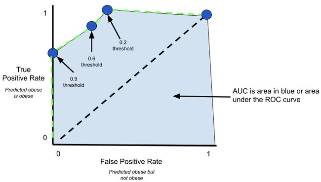
Here is an example of a ROC curve (green line), notice the true positive rate (actually obese and predicted as obese) on the y-axis and false positive rate (non-obese but predicted as obese) on the x-axis. Finally, remember an ROC is used to summarize the TP rate and the FP rate at various thresholds. The curve wouldn’t show you the thresholds but it will show you what your false-positive rate will be at various true positive rates.

这是一个ROC曲线(绿线)的示例，请注意y轴上的真实阳性率(实际上是肥胖且预测为肥胖)和x轴上的假阳性率(非肥胖但预测为肥胖)。 最后，请记住，ROC用于总结各种阈值下的TP速率和FP速率。 曲线不会显示您的阈值，但会显示您在各种真实阳性率下的假阳性率。

真实正利率 (True Positive Rate)

True Positive Rate=TP/(TP+FN) 真实正利率= TP /(TP + FN)

误报率 (False Positive Rate)

False Positive Rate=FP/(FP+TN) 误报率= FP /(FP + TN)

Let’s quickly compare 3 separate thresholds on the ROC curve. A threshold of 0.9 has the following confusion matrix from which we can calculate a TP rate of 0.6 and a FP rate of 0.

让我们快速比较ROC曲线上的3个独立阈值。 阈值0.9具有以下混淆矩阵，从中可以计算出TP率为0.6和FP率为0。

Let’s plot the TP rate and FP rate points on our ROC curve. Let’s also plot the TP and FP rates for thresholds of 0.6 and 0.2 for demonstration.

让我们在ROC曲线上绘制TP速率和FP速率点。 我们还绘制了阈值0.6和0.2的TP和FP速率进行演示。

The green dashed line represents the ROC curve. The individual blue points are the result of 4 separate confusion matrixes where the threshold was adjusted. Now ask yourself, “If this was the cancer example and you wanted to make sure you captured/predicted all actual cancer diagnoses, which threshold would you choose?”

绿色虚线表示ROC曲线。 各个蓝点是调整阈值的4个单独的混淆矩阵的结果。 现在问自己：“如果这是癌症的例子，并且您想确保捕获/预测了所有实际的癌症诊断，那么您会选择哪个阈值？”

If you said 0.2 you are correct! At this threshold, your TP rate is 100% which means you’re capturing/predicting all actual cancer diagnoses. Your FP rate is ~0.33 which means your model is misclassifying some non-cancer diagnoses as having cancer but that’s alright. Scaring someone and having them spend the money to get tested carries fewer consequences than telling someone they don’t have cancer when they do.

如果您说0.2，那是正确的！ 在此阈值下，您的TP率为100％，这意味着您正在捕获/预测所有实际的癌症诊断。 您的FP率为〜0.33，这意味着您的模型将某些非癌症诊断错误地归类为患有癌症，但这没关系。 吓someone某人并让他们花钱进行测试所带来的后果要比告诉某人没有癌症时要少。

Now the ROC simply connects each point to help with visualizing threshold move from very conservative to more lenient. Finally, the ROC curve helps with visualizing the AUC.

现在，ROC只需将每个点连接起来，以帮助可视化阈值从非常保守到更宽松的变化。 最后，ROC曲线有助于可视化AUC。

So what is the Area Under the Curve (AUC)?

那么，曲线下面积(AUC)是多少？

You will often see a ROC graph with many ROC curves and each curve is a different classifier (ie. log regression, SVC, decision tree, etc.). AUC is a great simple metric that provides a decimal number from 0 to 1 where the higher the number the better is the classifier. AUC measures the quality of the model’s predictions across all possible thresholds. In general, AUC represents the probability that a true positive and true negative data points will be classified correctly.

您经常会看到具有许多ROC曲线的ROC图，并且每个曲线都是不同的分类器(即，对数回归，SVC，决策树等)。 AUC是一种非常简单的度量标准，它提供从0到1的十进制数字，其中数字越大，分类器越好。 AUC在所有可能的阈值范围内衡量模型预测的质量。 通常，AUC代表正确正负数据点正确分类的概率。

我们如何调整阈值？ (How Can we Adjust the Threshold?)

# Adjusting the threshold down from 0.5 to 0.25
# Any data point with a probability  of 0.25 or higher will be 
#  classified as 1. clf = LogisticRegression()
clf.fit(X_train, y_train)
THRESHOLD = 0.25
y_pred = np.where(clf.predict_proba(X_test)[:,1] >= THRESHOLD, 1, 0)
y_pred_proba_new_threshold = (clf.predict_proba(X_test)[:,1] >= THRESHOLD).astype(int)

Logistic regression does not have a built-in method to adjust the threshold. That said since we know by default the threshold is set at 0.50 we can use the above code to say anything above 0.25 will be classified as 1.

Logistic回归没有内置的方法来调整阈值。 就是说，由于我们默认情况下知道阈值设置为0.50，因此我们可以使用上述代码将0.25以上的值归为1。

结论 (Conclusion)

I hope I was able to help clear up some confusion when it comes to classification metrics. I found that keeping all the terms (ie. recall, precision, TP, TN, etc.) clear in your mind is easier when they are memorized using one particular example (ie. cancer diagnoses).

我希望我能够帮助消除有关分类指标的困惑。 我发现，使用一个特定的例子(例如癌症诊断)记住这些术语时，将所有术语(例如，回忆，精确度，TP，TN等)清晰地记住会更容易。

Feel free to offer your feedback and thanks for reading.

随时提供您的反馈，并感谢您的阅读。

翻译自: https://towardsdatascience.com/classification-metrics-thresholds-explained-caff18ad2747

机器学习 二分类分类阈值