Deeplizard pytorch课程学习笔记

lesson1 PyTorch Prerequisites - Syllabus（课程大纲） For Neural Network Programming Course

本章主要介绍了课程包含的内容以及到课程的最后掌握的知识

lesson2 Pytorch - Python Deep Learning Neural Network API

PyTorch is a deep learning framework and a scientific computing package

PyTorch的tensors以及相关的操作与 Numpy的n维数组十分相似。
Tensors对于深度学习来说十分重要，因为他是我们在搭建和训练神经网络时用到的数据结构。

关于PyTorch一些简短的历史：
2016年10月份PyTorch最初的版本发布了，在其发布之前，有一个框架叫做Torch。Torch是一个存在了一段时间的机器学习框架，基于Lua语言。
PyTorch很多开发者同时也是Torch的开发者。
Torch慢慢过时，一个基于python的新版本被需要，PyTorch就出现了。
PyTorch属于Facebook，但是除了Soumith这个创造者之外，还有很多其他的人做出了自己的贡献。

PyTorch的一些深度学习特点

PyTorch对于深度学习的优势在哪？
After understanding the process of programming neural networks with PyTorch, it’s pretty easy to see how the process works from scratch in say pure Python. This is why PyTorch is great for beginners.

After using PyTorch, you’ll have a much deeper understanding of neural networks and the deep learning. One of the top philosophies of PyTorch is to stay out of the way, and this makes it so that we can focus on neural networks and less on the actual framework.

总结一下，PyTorch仅提供必要的API，你需要几乎从头设计神经网络，这可以帮助你更好的理解深度学习，而不仅仅是依赖框架。

一个使得PyTorch流行的很大原因是利于研究，它使用动态计算图，计算图是随着操作被创造及时生成的。

使用PyTorch的第一个项目是搭建一个卷积神经网络在Fashion-MNIST数据集上来进行图像分类。

这个数据集包含了60000个训练样本二，十个衣服的分类

lesson3 PyTorch install - Quick and Easy

首先安装Anaconda科学套件组，然后登录PyTorch的官网根据自己的develpoment environment来选择PyTorch的版本。无需额外另装cuda，它将会和PyTorch一起安装。
验证PyTorch是否安装成功
1.To use PyTorch we import torch
2. To check the version, we use torch.version
3. to verity our GPU capabilities,we use torch.cuda.is_avaliable()
4. To check the cuda version torch we use torch.version.cuda

lesson4 Why Deep Learning And Neural Networks Use GPUs

这节课的目标：什么是cuda？cuda如何适应PyTorch？为什么要在神经网络训练的时候使用GPU？
Graphics Processing Unit（GPU）
GPU擅长处理特殊计算，当计算可以并行的时候GPU比CPU快得多。
对于一个给定的处理器来说，CPU通常有四核，八核或者十六核可以做并行计算，而GPU往往有上千个。所以一个并行执行的任务来说，使用GPU可以加快计算速度。

那么为什么GPU特别适合用于深度学习呢？因为神经网络本身就是高度并行（embarrassingly parallel）的任务，它由许多互相独立的小任务组成（例如卷积），
直观上，卷积核像一个滑动窗口在输入张量上滑动，实际上大部分的计算操作是同时被完成的，因为它们并不互相依赖。
Nvidia是一家专门生产GPU的公司，GPU是硬件，Nvidia为了帮助开发者们使用GPU强大的并行计算能力，发布了CUDA这个软件。CUDA为开发者们提供了API操控GPU，cuDNN是个特殊的库，the CUDA Deep Neural Network library

PyTorch中嵌入了CUDA，所以关于控制并行计算的一些CUDA API我们无需知道
如何在PyTorch中使用CUDA呢？

> t = torch.tensor([1, 2, 3])
> t
tensor([1,2,3])
#张量对象被这种方式创建时，默认运行在CPU上
> t = t.cuda()
> t
tensor([1,2,3],device='cuda:0')
#张量对象调用了cuda()以后，它的一系列计算就会在GPU上
#PyTorch这种可以控制计算在CPU还是GPU上的能力十分versatile

并不是所有的运算都应该在GPU上进行，因为将数据从CPU上传送到GPU上的代价挺大的，当任务不是很复杂的情况，使用CPU反而更加，当我们真正需要的时候再使用GPU。

lesson5 Introducing Tensors For Deep Learning

A tensor is the primary data structure used by neural networks

number,array,2d-array时计算科学里的名词，scalar，vector，matrix是数学中的名词
在深度学习中这些术语都被称为向量
上述不同领域中的术语其实是一一对应的

• number,scalar
• array,vector
• 2d-array,matrix

在深度学习中，Tensors and nd-arrays are the same thing!

• A scalar is a 0 dimensional tensor
• A vector is a 1 dimensional tensor
• A matrix is a 2 dimensional tensor
• A nd-array is an n dimensional tensor
  n描述了该张量有多少个维度，在指定一个特定的元素时需要n个索引，利用0维张量不需要索引，可以directly use

向量和张量的区别，n维向量只能包含n个component，而n维张量可以包含任意个component

Lesson6 Rank,Axes And Shape -Tensor For Deep Learning

Rank of A Tensor

The rank of a tensor refers to the number of dimensions present within the tensor.We have a rank-2 tensor意味着我们拥有一个矩阵，一个二维数组，或者二维张量
A tensor’s rank tells us how many indexes are needed to refer to a specific element within the tensor

Axes of a Tensor

当我们拥有一个张量的时候，想要指定它的一个特定的维度，使用axis这个术语来表示。
An axis of a tensor is a specific dimension of a tensor

Shape of a Tensor

The shape of a tensor gives us the length of each axis of the tensor

> t = torch.tensor([[1,2,3],[4,5,6]])
> t.shape
torch.Size([2,3])

我们做为一个写代码的人，能够理解输入张量的形状，并且在需要的时候reshape
reshape前后的元素个数应该一样
Reshaping changes the shape but not the underlying data elements

> t = torch.tensor([[1,2,3],[4,5,6]])
> t.shape
torch.Size([2,3])
> t = t.reshape(3,2) #不是原地改变张量，而是有一个返回值
> t.shape
torch.Size([3,2])

Lesson 7 CNN Tensor Input Shape And Feature Maps

A practical example that demonstrates the use of the tensor concepts rank, axes and shape
CNN的输入通常是个rank-4的tensor，（batch,channels,height,width）
Given a tensir of images like this, we can navigate to a specific pixel in a specific color channel of a specific image in the batch using four indexes
当输入张量经过卷积层运算以后颜色通道axis的意义就会发生变化
height width的大小的会因为卷积核的尺寸，步长，padding而改变
color channel的数量由卷积核的数量来决定。
Feature maps are the output channels created from the convolutions.

lesson 8 PyTorch Tensors Explained - Neural Network Programming

PyTorch tensors are the data structure we’ll be using when programming neural networks in PyTorch
当进行神经网络编程的时候，数据预处理往往是整个过程的第一步，数据预处理大的一个目标就是将未处理过的数据变成tensor的形式。

> t = torch.Tensor()
> type(t)
torch.Tensor

PyTorch中的所有tensor对象都有三个属性dtype，layout，device

> t = torch.Tensor()
> t.dtype
> t.device
> t.layout
torch.float32
cpu
torch.strided

tensor.dtype

张量之间能够运算的前提是数据类型相同（PyTorch1.3以下）

torch.tensor([1],dtype=torch.int) + torch.tensor([1],dtype=torch.float32)

这在1.3以下的版本不允许，1.3及以上会得到一个dtype为torch.float32的张量

> device = torch.device("cuda:0")
> device
device(type='cuda',index=0)

PyTorch支持使用多个设备，通过上面这种索引的方式来分配。如果两个张量之间需要进行运算，那么它们必须得在同一个设备上，在创建一个实例对象时可以通过将设备传入构造器来指定

t = torch.tensor([1],device = device)
tensor([1],device='cuda:0')

用tensor来得到张量对象时，不能为空，而Tensor可以创建空数据的tensor对象

注意点：

1. Tensors contain data of a uniform type(dtype)
2. Tensor computations between tensors depend on the dtype and the device

Creating Tensors Using Data

• torch.Tensor(data)
• torch.tensor(data)
• torch.as_tensor(data)
• torch.from_numpy(data)
  这四个方法都可以接收一定形式的data，data是一个array-like的数据，然后返回一个torch.Tensor类的实例
  
  torch.eye(2) 返回一个2-D tensor单位矩阵
  torch.zeros([2,2]) 返回一个指定shape的0张量
  torch.ones([2,2])返回一个指定shape的全为1的张量

Lesson 9 Creating PyTorch Tensors - Best Options

上述四种创建tensor对象的方式有什么不同？哪一个更好？

torch.Tensor() VS torch.tensor()

torch.Tensor()是一个构造函数，torch.tensor()是一个factory function返回一个torch.Tensor
的对象。
torch.tensor() 拥有更好的文档核更多的配置选项

torch.Tensor()的dtype使用的时torch.get_default_dtype(),一般是浮点类型，其它三种方法的dtype取决于输入数据的类型。
torch.tensor(),torch.as_tensor()可以传入dtype来指定，而Tensor构造函数不可以传dtype

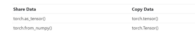
原始数据改变时，由原始数据得到的tensor，如果是share data的话会跟着改变。这种共享使用的内存会更小，并且可以通过t.numpy()返回一个ndarray的对象。
torch.from_numpy()只能接收numpy.ndarray,而as_tensor可以接收array-like object甚至其他的tensor对象。

最好的option
torch.tensor()
torch.as_tensor()

lesson 10 Reshaping Operations - Tensors For Deep Learning

知道了一个tensor的shape以后，可以推测出一系列的东西。首先，可以得到tensor的rank。
The rank of a tensor is equal to the length of the tensor’s shape
知道了shape，还可以得到这个张量所包含的element的个数，当然也可以直接调用一个简单的方法

t.numel()

改变一个tensor的shape同样可以使用Squeezing 和 Unsqueezing

Squeezing a tensor removes the dimensions or axes that have a length of one

> t = torch.tensor([[1,2,3,4,5,6]])
> t.size() # size is exactly same to shape in PyTorch
tensor.Size([1,6])
> t.squeeze()
tensor([1,2,3,4,5,6])
> t.size()
tensor.Size([1,6])

tensor.Squeeze()返回一个压缩后的tensor，不改变原来的变量tensor.Unsqueeze(dim=n)
在第n-1个位置扩展一个长度为1的axis

> t = torch.tensor([1,2,3,4])
> t.unsqueeze(dim = 1)
tensor([[1],
         [2],
         [3],
         [4]])
 > t.unsqueeze(dim = 0)
 tensor([[1,2,3,4]])

还有一种改变tensor的shape的一个方法叫做flatten

Flattening a tensor means to remove all of the dimensions except for one

def flatten(t):
	t = t.reshape(1,-1)
	t = t.squeeze()
	return t

the - 1 tells the reshape() function to figure out what the value should be based one the number of elements contained within the tensor.

Concatenating Tensors

用cat(（t1,t2,…）,dim=) 方法在指定的轴上拼接若干个张量

> t1 = torch.tensor([1,2,3])
> t2 = torch.tensor([4,5])
> t3 = torch.tensor([6])
> torch.cat((t1,t2,t3),dim = 0) #这里张量都是一维的，所以只能在一维上拼接
tensor([1,2,3,4,5,6])
>t4 = torch.tensor([[1,2,3]])
>t5 = torch.tensor([[4,5]])
>torch.cat((t4,t5),dim = 1)
tensor([[1,2,3,4,5]]) #注意这里只能在列上拼接

Lesson 11 CNN Flatten Operation Visualized - Tensor Batch Processing For Deep Learning

tensor.flatten()
tensor.reshape(1,-1).squeeze()

都可以将一个张量展成一维，但是怎么去展平一个特定的张量轴呢？
一个卷积神经网络通常右4个轴：（Batch Size，Channels，Height，Width）
如果我们想保留batch的信息，只是将后三个轴展平，通过flatten依然可以办到。

t.flatten(start_dim = 1)#表示从序号为1的轴往后展平

Lesson 12 Tensors Fo Deep Learning - Broadcasting And Element-wise(元素层面) Operations With PyTorch

Element-wise 意味着什么？

An element-wise operates on corresponding elements between tensors
corresponding 意味着两个元素在张量中占据着相同的位置

t1 = torch.tensor([
	[1,2],
	[3,4]
],dtype=torch.float32)
t2 = torch.tensor([
	[9,8],
	[7,6]
],dtype=torch.float32)
t1[0][0] = 1
t2[0][0] = 9
就是两个corresponding的element

tensors之间必须有着同样数量的元素（exactly same shape）才能具有element-wise operation,操作以后shape不变

加法就是一个element-wise的操作

 > t1 + t2
 tensor([
	[10.,10.],
	[10.,10.]
])

实际上，加法，减法，除法，乘法都是element-wise的operation

张量和标量进行算术运算时，标量会与张量中的每一个位置的元素进行运算。

> t + 2
> t.add(2)
> 
> t - 2
> t.sub(2)
>
> t / 2
> t.div(2)
> 
> t * 2
> t.mul(2)

Broadcasting Tensors

Broadcasting is the concept whose implementation allows us to add scalars to higher dimensional tensors.
t + 2这个操作，标量2首先被broadcasting到了t的shape，然后element-wise操作被执行
比较同样是一种element-wise操作
对于给定两个张量之间的比较操作，会返回一个相同的tensor包含了torch.value of True or False

> torch.tensor([1,2,3]) < torch.tensor([2,1,6])
tensor([True,False,True])

一些常见的比较函数（element-wise）

> t.eq(number)#是否和number相同
> t.ge(number)#是否大于等于number
> t.gt(number)#是否大于number
> t.le(number)#是否小于等于number
> t.lt(number)#是否小于number

一些常见的elment-wise操作

t.abs()#绝对值
t.sqrt()#开方
t.neg() #取负数

lesson 13 Code For Deep Learning - ArgMax And Reduction Tensor Ops

A reduction operation on a tensor is an operation that reduces the number of elements ccontained within the tensor
Tensors拥有管理数据的能力
Reshaping operations给了我们沿着特定轴position elements的能力。Element-wise允许我们在两个tensor之间操作，reduction operation允许使得我们在单一张量内操作。

t = torch.tensor([
	[0,1,0],
	[2,0,2],
	[0,3,0]
],dtype=torch.float32)

> t.sum()
tensor(8.)
> t.numel()
9
>t.sum().numel()
1
#由于元素的数量减少了，我们可以总结出sum是一个reduction操作
> t.mean()
tensor(.8889)
> t.std()
tensor(1.1667)
> t.prod()
tensor(0.)

reduction operations不一定总是将一个tensor缩减到一个单独的元素，可以让tensor沿着特定的轴进行缩减

t = torch.tensor([
	[1,1,1,1],
	[2,2,2,2],
	[3,3,3,3]
],dtype=torch.float32)
> t.sum(dim = 0)
tensor([6.,6.,6.,6.])
> t.sum(dim = 1)
tensor([4.,8.,12.])
#指定的轴进行缩减，dim=0，将三个数组变成一个数组，所以对应位置应该相加
> t[0] + t[1] + t[2]
> [6,6,6,6] -->Element-wise operations are in play here
> t[0].sum()
> tensor(4.)
> t[1].sum()
> tensor(8.)
> t[2].sum()
> tensor(12.) #sum将一个数组缩减成一个标量

Argmax Tensor Reduction Operation

Argmax returns the index location of the maximum value inside a tensor

> t = torch.tensor([
	[1,0,0,2],
	[0,3,3,0],
	[4,0,0,5]
],dtype = torch.float32)
> t.max()
tensor(5.)
> t.argmax()
tensor(11.)

tensor.max方法返回了t中的最大值，argmax如果不指定特定的轴的话，会返回张量被展平以后最大值所对应的索引。

> t = torch.tensor([
	[1,6,3,8],
	[3,2,7,9],
	[6,0,8,3]
])
> t.max(dim = 0)
torch.return_types.max(
	values=tensor([6,6,8,9]),
	indices=tensor([2,0,2,1])
)
> t.argmax(dim=0)
tensor([2,0,2,1])

在指定特定的轴以后max返回的是对该轴进行element-wise操作的最大值以及该值对应的索引。argmax在指定轴以后，返回的就是对应的索引。
实际应用场景中，我们通常使用argmax作用在一个神经网络的output prediction tnsor上，来决定哪一个种类拥有最高的预测值。

> t = torch.tensor([
	[1,2,3],
	[4,5,6],
	[7,8,9]
],dtype=torch.float32)
> t.mean()
tensor(5.)
#返回的是一个0维张量，如果我们想得到具体的值使用item方法
> t.mean().item()
5.0
> t.mean(dim=0).tolist()
[4.,5.,6.]
> t.mean(dim=0).numpy()
array([4,5,6],dtype=float32)
#可以将一维张量变成list或者numpy
#tensor支持numpy中绝大多数的切片和索引操作

Lesson 14 Dataset For Deep Learning - Fashion MNIST

Index	Label
0	T-shirt/top
1	Trouser
2	Pullover
3	Dress
4	Coat
5	Sandal
6	Shirt
7	Sneaker
8	Bag
9	Ankle boot

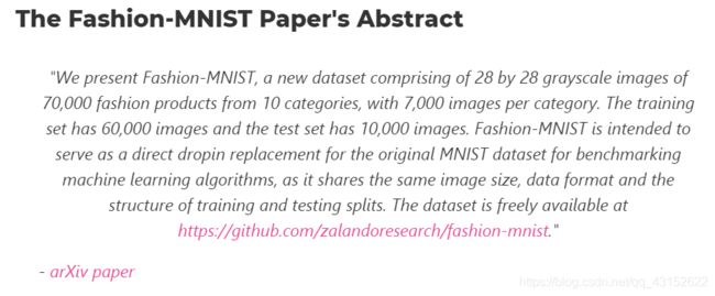
torchvision这个library包括了MNIST和Fashion-MNIST

Lesson 15 CNN Image Preparation Code Project - Learn To Extract, Transform, Load(ETL)

prepare the data

为了准备我们的数据，我们遵循的叫做ETL过程

1. Extract data from a data source
2. Transform data into a desirable format.
3. Load data into a suitable structure
   ETL过程可以被看作是一种fractal process

Package	Description
torch	the top-level PyTorch package and tensor library
torch.nn	A subpackage that contains modules and extansible classes for building neural nerwork
torch.optim	A subpackage contains standard optimization operations like SGD,Adam
torch.nn.functional	A functional interface that contains typical operations used for building networks like loss functions and convolutions
torchvision	A package that provides access to popular datasets,model architectures,image transformations for computer vision
torchvision.transforms	An terface that contains common transforms for image processing

使用PyTorch来准备我们自己的数据

1. Extract - Get the Fashion-MNIST image data from the source
2. Transform-Put the data into tensor form
3. Load - Put our data into an object to make it easily accessible.

Class	Description
torch.utils.data.Dataset	An abstract class for representing a dataset
torch.utils.data.DataLoader	Wraps a dataset and provides access to the underlying data

我们可以创建一个自己的数据库，通过创建一个继承Dataset方法的子类
这个新的子类可以被传给一个DataLoader对象。

torchvision包

可以为我们提供Datasets(例如MNIST和Fashion-MNIST)
可以提供一些经典的模型（like VGG16）
Transforms还有utils

train_set = torchvision.datasets.FashionMNIST(
	root='./data',
	train=True,
	download=True,
	transform=transforms.Compose([
		transforms.ToTensor()
	])
)

参数	介绍
root	数据在哪里被下载
train	数据集是否是训练集
download	数据是否应该被下载
transform	应当对数据集元素执行的转换的组合

只有在第一次被执行是才会下载数据，是数据集所以train设为True，我们想要自己的image被转换成tensor，所以使用了内置的transforms.ToTensor()

train_loader = torch.utils.data.DataLoader(train_set,batch_size=1000,shuffle = True)

Lesson 16 Training Set Exploration For Deep Learning And AI

本章内容主要是深度了解Dataset 和 DatasetLoader这两个Class，了解训练集

working with the training set

> len(train_set)
60000
> train_set.targets
tensor([9,0,0,...,3,0,5])
> train_set.targets.bincount()
tensor([6000,6000,6000,6000,6000,6000,6000,6000,6000,6000])

len()方法可以获得训练集中样本的个数，targets属性可以得到对应样本的labels，bincount()可以查看每种lable对应的数目。
Class imbalance 是一个普通的问题，但是Fashion-MNIST dataset是balance的

为了得到训练集中一个单独的元素，我们首先把train_set对象传入到Python的**iter()**中，它将返回一个代表一连串数据的对象。
**next()**方法可以逐个迭代数据流中的数据

> sample = next(iter(train_set))
> type(sample)
tuple
> len(sample)
2
> image,label = sample
> type(image)
torch.Tensor
> image.shape
torch.Size([1,28,28])
> type(label)
int

得到的sample是包含两个元素的元组，第一个元素是tensor,shape为（1，28，28）颜色通道为1（gray）宽高各位28的像素数据,第二个元素是这个图片对应的label。

import matplotlib.pyplot as plt
plt.imshow(image.squeeze(),cmap='gray')

working with Batches of Data

> display_loader = torch.utils.data.DataLoader(
	train_set,batch_size = 10
)

DataLoader提供shuffle这个参数，默认情况下shuffle为False，一个epoch结束后不进行打乱。

batch = next(iter(display_loader))
images,labels = batch
type(images) type(labels)
torch.tensor   torch.tensor
images.shape
torch.Size([10,1,28,28])

tensor的大小取决于batch_size
下面我们尝试来可视化这批图像数据

grid = torchvision.utils.make_grid(images,nrow=10)
#make_grid接收四维张量，用于做图像之间的拼接，nrow代表一行显示多少个图片，#padding默认为2
grid.shape
torch.Size([3,32,302])
#宽在横向上被拼接到了一块，再加上图片之间的padding 28 * 10 + 9 * 2 = 302

这里第一轴的长度为3，我的理解是颜色通道数，原本只有一个颜色通道的灰度图像，沿着颜色通道重复了三次,对于imshow来说三通道相等的灰度值，它好像可以自动识别为灰度图像，下面是我做的一个实验

> image.shape
torch.Size([1,28,28]) #image是单个灰度图像
> test = torch.stack((image,image,image))
torch.Size([3,1,28,28])
> plt.imshow(numpy.transpose(test.squeeze().numpy(),(1,2,0)))
#test.squeeze先将长度为1的轴压缩掉变成[3,28,28]
#numpy()将张量转换成numpy数组，这样可以使用numpy.transpose对其进行转置
#转置结果为[28,28,3] H * W * C符合imshow的绘图数据格式
> plt.imshow(image,cmap='gray')
#实验结果发现二者的绘制图像一摸一样

plt.imshow(grid.permute((1,2,0)))

这里是用permute对[3,32,302]进行轴对调 [32,302,3]注意不能直接用reshape

How to Plot Images Using PyTorch

how_many_to_plot = 20
train_loader = torch.utils.data.DataLoader(
	train_set,shuffle=True,batch_size=1
)
for i,batch in enumerate(train_loader,start=1):
	image,label = batch
	plt.subplot(10,10,i)
	plt.imshow(image.squeeze(),cmap='gray')
	plt.axis('off')
	plt.title(train_set.classes[label.item()],fontsize=28)
	if(i >= how_many_to_plot):break
plt.show()

这里注意几点，enumerate中的start = 1表示i从1开始，plt.axis(‘off’)表示不显示坐标轴。
train_set.classes中记录了所有标签的名字

Lesson 17 Build PyTorch CNN - Object Oriented Neural Networks

本节将开始搭建第一个CNN
上面几节已经网络第一步Prepare the data，下一步就开始build the model
因为开始这一章需要有object oriented programming的知识，所以先进行面向对象编程的学习。

Classes是一种将data和functionality绑定在一起的方法。每个Class的实例（instance）可以拥有一些属性（attribute）来保持它的状态（state），同样也可以拥有一些方法（methods defiend by its class）来改变实例本身的状态。

oop

namespace是一种从名字到对象的映射。大多数的namespace都是一个python的字典，通常不可见，并且可以发生变化。有一些关于namespace的例子：内置（built-in）的名字集合，比如abs()这样的函数；模块中的全局变量；函数局部的变量；某种意义上一个对象的属性也构成了一个命名空间。不同命名空间里的名称没有联系。
attribute的含义，只要一个name后面跟着一个dot，比如z.real,real就是z的attribute，这对于模块中的名称引用也是一样的。attribute可以是只读的也可以是可写的，对于writeable的attribute可以通过del modelname.name进行删除。
不同时刻创建的namespace拥有不同的生命周期。比如包含内置函数的命名空间在Python的解释器启动时就被创建了，并且从未被删除。一个模块的全局命名空间在定义被读入时就被创建了，通常引入模块的命名空间也持续到解释器退出.

scope决定了怎么查找namespace
首先找一个name时，从最内部的局部变量开始找，然后再找nonlocal，再找global。global可以在任何地方修饰一个变量，但是不能直接赋值。nonlocal只能在嵌套函数中使用，表示是外层嵌套函数的局部变量。

类对象支持两种操作：attribute references和instantiation（实例化）
合法的属性名称是那些存在于class的namespace中的

class MyClass:
	“”“A simple example class”“”
	i = 12345
	def f(self):
		return "hello world!"

MyClass.i和MyClass.f就是合法的attribute references,__doc__同样也是一个合法的属性，它会返回“A simple example class”

Class instantiation使用了函数的符号，可以假装class object是一个没有参数的函数，它返回一个类的新实例

x = MyClass()

许多类在实例化的时候会创建一个特殊的状态，因此一个类可能会定义一个特殊的方法叫做__init__(),在类实例化操作时传入的参数会被传递给__init__函数

class Complex:
	def __init__(self,realpart,imagpart):
		self.r = realpart
		self.i = imagpart
x = Complex(3,4)
x.r,x.i
==>3，4

一个实例化的对象拥有两个合法的属性成员：data atrributes和methods。
对于data attribute而言不一定需要被声明，在第一次被分配值时就存在了，当然，可以通过del删除

x.counter = 1
while x.counter < 10:
	x.counter = x.counter * 2
print(x.counter)
del x.counter

一个对象合法的方法名取决于它的类。

MyCLass.f(x) ==  x.f()

实例对象通常会被当作函数的第一个参数传入，所以上面两种调用方法的方式效果一样，
通常来说，实例变量是为了每一个实例与众不同，类的变量是被类中共享的属性和方法。
对于列表和字典来说，它们要是成为了类的属性，那么会被所有实例化的对象共有，因为它们拿到的引用相同。

class Dog:
	tricks = []
	def __init__(self,name):
		self.name = name
#这个trick会被所有instance持有，一个改变所有都改变
> x = Dog('one')
> y = Dog('two')
> x.tricks.append(5)
此时x.tricks和y.tricks都变成[5]
class Dog:
	def __init__(self,name):
		self.name = name
		self.tricks = []
#正确做法是给每一个对象都分配一个

如果对象的属性和类的属性名称一样时，对象属性的查找要优先,注意类的属性依然存在

class Dog:
	tricks = [5]
	def __init__(self,name):
		self.name = name
> x = Dog('one')
> y = Dog('two')
> y.tricks = [] #此时x.tricks依然是[5],
> del y.tricks
> y.tricks
> [5] #类的属性依然存在，不会被对象属性覆盖

继承这个概念对于面向对象编程来说十分重要

class DerivedClassName(BaseClassName):
	<statement-1>
	...
	<statement-N>

如果一个被需求的属性在类中没被找到，那么就会在被继承的类中查找，这个查找过程是迭代的。继承的类可以重写基类的方法。
isinstance(obj,int)可以检查obj.__class__是否是int或者从int继承的其他类。
issubclass(bool,int)检查bool是否是int的子类，返回True

多继承

class DerivedClassName(Base1,Base2,Base3):
	<statement-1>
	...
	<statement-N>

查找属性时是深度优先，而后从左到右

PyTorch’s torch.nn Package

为了在PyTorch上创建neural networks，我们使用torch.nn这个包，这里的nn代表neural network。nn这个库包含了构建神经网络的一些经典组件。
建造神经网络最主要的组件就是layer，nnlibrary中包含了一些能够帮助我们建造层的classes。
每一层包括了两个主要的组件：
1.A transformation(code)
2.A collection of weights(data)
这个transformation可以理解为从输入到输出的变换，无论是前向计算还是反向传播，都是对state的一种改变
A collenction of weights就相当于neural nerwork内部维护的数据
既有自身的状态又有改变状态的方法，neural network就很适合oop。
nn包里就有一个类叫做Module，它是所有包含layer的基类，即任何的layer都得继承nn.Module这个类，继承了nn.Module中的所有函数。neural network也需要继承自nn.Module，因为一个nn本身可以看作一个大的layer。
当我们给network传递一个tensor作为输入时，tensor 向前传递并经过每一层的变换最终到达输出层。这个过程被称为forward pass。nn中所有layer的transformation可以看成一个大的transformation，这也是为什么一个nn可以被看作一个大的layer。
nn.Module拥有一个forward方法，所以当我们建一个layer或者是nn时，必须提供一个forward（）方法，它代表了真正的变换。
nn.functional包中提供我们在transformation中需要的方法。

Building A Neural Network In PyTorch

outline:

1. create a neural network class that extends the nn.Module base class
2. In the class constructor,define the network’s layers as attributes using pre-built layers form torch.nn
3. Use the network’s layer attributes as well as operations from the nn.functional API to define the network’s forward pass
   下面看一个dummy example

class Network(nn.Module):
	def __init__(self):
		super().__init__()
		self.layer = None
	def forward(self,t)
		t = self.layer(t)
		return t

forward中传入一个张量，并将其送入layer中进行transformation，得到一个新的张量返回，最后的输出结果也是一个张量。

class Network(nn.Module):
	def __init__(self):
		super().__init__()
		self.conv1 = nn.Conv2d(in_channels=1,out_channels=6,kernel_size=5)
		self.conv2 = nn.Conv2d(in_channels=6,out_channels=12,kernel_size=5)
		self.fc1 = nn.Linear(in_features=12*4*4,out_features=120)
		self.fc2 = nn.Linear(in_features=120,out_features=60)
		self.out = nn.Linear(in_features=60,out_features=10)
	def forward(self,t):
		#implement the forward pass
		return t

Lesson 18 CNN Layers - PyTorch Deep Neural Network Architecture

我们使用到的nn下面这些class都是继承自Module，它们都包含两个重要的部分，a forward function 和 a weight tensor
每个layer中包含的weight tensor它们都会随着训练过程而update。
parameter和argument这两个都有参数的意思，但parameter代表的是形参，argument代表的是实参。
Convolutional layers拥有三个parameters
in_channels,out_channels,kernel_size
Linear layers拥有两个parameters
in_features,out_features
通常情况下，hyperparameters(超参数)是那些手动地，任意地指定值的参数。我们选择超参数往往是根据实验结果或者是往常的经验。对于CNN来说，下面是需要手工指定的parameters

Parameter	Description
kernel_size	Sets the fileter size.The words kernel and filter are interchangeable
out_channels	Sets the number of filters.One filter produces one output channel
out_features	Sets the size of the output tensor

Data Dependent Hyperparameters的value取决于数据.第一层的卷积层的in_channels取决于images的颜色通道数，由于是灰度图像所以被设置为1.输出层的out_features取决于类的数量。通常情况下，一层的输入是上一层的输出，所以所有conv_layers的in_channels和linear layers的in_features取决于上一层来的数据。

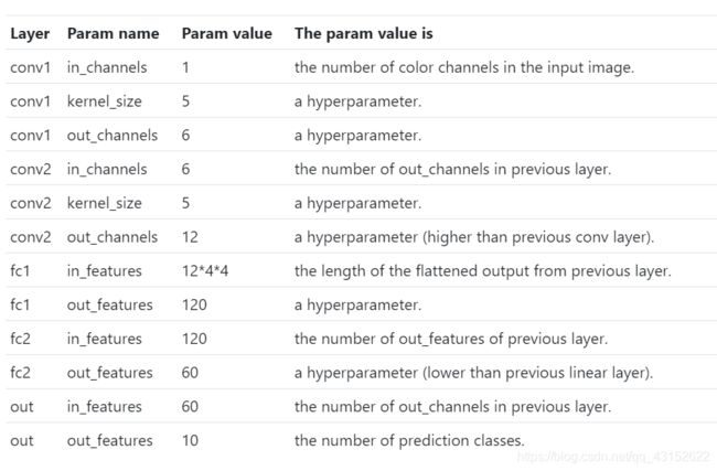
channels就是卷积核的数量，features就是本层神经元个数。

Lesson 19 CNN Weights - Learnable Parameters In PyTorch Neural Networks

Learnable parameters are parameters whose values are learned during the training process.这些可学习的参数通常是从一些随机值开始，这些可学习的参数就是nn中的weights tensor，它们存在于每一层当中。

Getting An Instance Of The Network

为了更加直观的查看weights，可以先创建一个Network的instance

> network = Network()
> print(network)
Network(
    (conv1): Conv2d(1, 6, kernel_size=(5, 5), stride=(1, 1))
    (conv2): Conv2d(6, 12, kernel_size=(5, 5), stride=(1, 1))
    (fc1): Linear(in_features=192, out_features=120, bias=True)
    (fc2): Linear(in_features=120, out_features=60, bias=True)
    (out): Linear(in_features=60, out_features=10, bias=True)
)

nn.Module重写了object的__repr__方法所以可以打印出网络结构的详细信息。这里的kernel_size是个tuple(5,5)因为fileters有宽和高，只传一个值默认是个方块stride可以自己设，默认的就是(1,1)
nn中的layer都是network对象的attribute，可以通过dot直接引用

network.conv1.weight
Parameter containing:
tensor([[[[ 0.0661, -0.0526,  0.0384, -0.1292,  0.1718],
          [-0.0504, -0.1117, -0.1118,  0.0549, -0.0404],
          [ 0.0527,  0.1913,  0.0698,  0.1465, -0.0032],
          [ 0.0422,  0.1443, -0.0420, -0.1730, -0.0563],
          [ 0.1047,  0.0675, -0.0774, -0.0310, -0.1093]]],

        [[[ 0.0224, -0.0661, -0.1269, -0.0029, -0.1507],
          [-0.0318,  0.1143,  0.1889, -0.0094, -0.0569],
          [ 0.1713,  0.0599, -0.0921, -0.0562,  0.0774],
          [-0.0118, -0.0443,  0.1729, -0.0111,  0.1596],
          [-0.1607, -0.0268,  0.0878, -0.1254,  0.1754]]],

        [[[-0.0976, -0.1594,  0.0759,  0.0562, -0.0597],
          [ 0.1001,  0.1000, -0.0359,  0.1469,  0.0771],
          [ 0.1260, -0.0936,  0.1957, -0.0606,  0.0254],
          [ 0.0380, -0.0957, -0.1091,  0.1820,  0.0693],
          [-0.1713, -0.1339, -0.1452, -0.1212, -0.0077]]],

        [[[-0.0695, -0.0719,  0.1501, -0.0411, -0.1044],
          [ 0.0192, -0.0260,  0.1304,  0.0117, -0.0785],
          [-0.0585, -0.1911,  0.0017, -0.0590,  0.0895],
          [-0.0607, -0.1362,  0.0125,  0.0836,  0.0236],
          [-0.1904,  0.1037, -0.1755,  0.0364, -0.0613]]],
          
        [[[ 0.0426,  0.0226, -0.1490, -0.0030,  0.0929],
          [-0.1535, -0.1069,  0.0991, -0.0761,  0.1754],
          [ 0.0357, -0.0326,  0.0242,  0.0985,  0.1372],
          [-0.1145, -0.1267, -0.0431, -0.1388, -0.1467],
          [-0.1254, -0.1186,  0.1287,  0.0250, -0.1835]]],
          
        [[[ 0.1285,  0.0279, -0.1453, -0.1030,  0.1383],
          [ 0.1237,  0.1846, -0.1898,  0.0009, -0.0589],
          [ 0.0269, -0.1861,  0.0582,  0.0622,  0.0567],
          [ 0.1883, -0.0467, -0.0261,  0.1460, -0.0023],
          [ 0.0399,  0.0799,  0.1258,  0.1771, -0.0900]]]], requires_grad=True)

可以发现weight是个张量，但是打印出来的格式和普通的张量不同。为了跟踪network中的weight tensor，PyTorch有个特殊的类叫做Parameter，Patameter是继承自tensor class，每个layer中的weight tensor都是Parameter类的一个实例.

> network.conv1.weight.shape
torch.Size([6,1,5,5])
> network.conv2.weight.shape
torch.Size([12,6,5,5])

卷积核组被实现成一个rank-4 tensor，第一个轴代表卷积核的个数，第二个代表卷积核的通道数，第三、四分别代表高度和宽度。

对于Linear layers，rank-1的tensor作为输入和输出，weight tensor是一个rank-2的matrix

> network.fc1.weight.shape
torch.Size([120,192]) = = > torch.Size([out_features,in_features]) 

Accessing The Networks Parameters

for param in network.parameters():

#如果同时想知道名字
for name,param in network.named_paramters():
	print(name,'\t\t',param.shape)

Lesson 20 Callable Neural Networks - Linear Layers In Depth

Transform Using A Matrix

对于linear layer来说，输入一个一维张量，做的变换就是一个weight matrix，把这个weight matrix与数量张量相乘，得到输出张量。

in_features = torch.tensor([1,2,3,4],dtype=torch.float32)
weight_matrix = torch.tensor([
    [1,2,3,4],
    [2,3,4,5],
    [3,4,5,6]
],dtype=torch.float32)
weight_matrix.matmul(in_features)
> tensor([30.,40.,50.])

nn.Linear可以得到和上面一样的效果，我们来构造一个linear的实例

in_features = torch.tensor([1,2,3,4])
fc = nn.Linear(in_features=4,out_features=3)
fc(in_features)
> tensor([-0.8877,1.4250,0.8370],grad_fn=<AddBackward0)

这里比较神奇的是fc作为一个对象，竟然直接可以被调用，类似这种直接被调用的object被称为callable Python objects。运算结果之所以这么奇怪是因为linear里面的weight matrix是被随机初始化的，你每调用一次，运算结果都可能不同。当然也可以直接传递weight matrix.

fc.weight = nn.Parameter(weight_matrix)
fc(in_features)
> tensor([30.2639,40.07569,50.1887],grad_fn=<AddBackward0)

weight必须等于一个nn.Patameter实例化的对象，可以发现结果已经与[30,40,50]十分接近了，之所以没有完全相等是因为有个bias

fc = nn.Linear(in_features=4,out_features=3)
fc.weight = nn.Parameter(weight_matrix)
fc(in_features)
> tensor([30.,40.,50.],grad_fn=<SqueezeBackward3)

把bias置为False就得到exact的结果了。
Mathematical Notation Of The Linear Transformation
$y=Ax+b$

Variable	Definition
A	Weight matrix tensor
x	Input tensor
b	bias tensor
y	output tensor

前面提到的callable object就是能够像函数一样被调用的object，在进行类定义的时候添加一个特殊的Python function叫做__call__,在object被call的时候就调用__call__这个函数。nn programming中我们并不是直接调用forward函数，而是调用函数本身，就像上面的nn.Linear一样，__call__这个函数中会间接调用forward

Lesson 22 CNN Forward Method - PyTorch Deep Learning Implementation

class Network(nn.Module):
	def __init__(self):
		super().__init__()
		self.conv1 = nn.Conv2d(in_channels=1,out_channels=6,kernal_size = 5)
		self.conv2 = nn.Conv2d(in_channels=6,out_channels=12,kernal_size=5)
		self.fc1 = nn.Linear(in_features=4 * 4 * 12,out_feaures=120)
		self.fc2 = nn.Linear(in_features=120,out_features=60)
		self.out = nn.Linear(in_features=60,out_feaures=10)
	def forward(self,t):
		t = self.conv1(t)
		t = F.relu(t)
		t = F.max_pool2d(t.kernal_size=2,stride=2)

		t = self.conv2(t)
		t = F.relu(t)
		t = F.max_pool2d(t.kernal_size=2,stride=2)

		t = t.flatten(start_dim=1)
		t = self.fc1(t)
		t = F.relu(t)

		t = self.fc2(t)
		t = F.relu(t)
			
		t = self.out(t)
		return t

最后不用使用softmax操作，因为loss function F.cross_entropy会隐式地对它的输入使用softmax，我们最后只返回一个线性变换的结果。

Lesson 23 CNN Image Prediction With PyTorch - Forward Propagation Explained

forward propagation is just a special name for the process of passing an input to the network and receiving the output from the network.

前向传播就是tesnsor在网络中前进时做的变换过程，下面进行一个图片的数据在网络模型中进行前向传播的过程。

import torch
import torchvision
import torchvision.transforms as transforms
import torch.nn as nn
import torch.nn.functional as F

train_set = torchvision.datasets.FashionMNIST(
	root='./',
	download=True,
	train=True,
	transform=transforms.Compose([
		transforms.ToTensor()
])
)
image,label = next(iter(train_set))
network = Network()
predict = network(image.unsqueeze(dim=0))
predict.shape
>tensor.Size([1,10])
predict = F.softmax(predict,dim=1)
predict.argmax()
>tensor(5)

Lesson24 Neural Network Batch Processing with PyTorch

这节的目的是往我们的网络中传入一个batch的图片，并且解释其结果。

train_loader = torch.utils.data.DataLoader(
	train_set,batch_size=10
)
images,labels = next(iter(train_loader))
def get_correct_nums(predict,labels):
	return predict.argmax(dim=1).eq(labels).sum().item()

predict = network(images)
get_correct_nums(predict)

eq是个element-wise的操作，比较两个张量对应位置是否相等，最后返回一个一样shape的bool张量。sum对结果进行reduct，最后转化成标量返回。

Lesson 25 CNN Output Size Formula - Bonus Neural Network Debugging Sesson

这节的主要内容是输入在CNN中如何进行transform的。
学习在VSCode中配置python环境，以及如何调试PyTorch代码。

Lesson 26 CNN Training With Code Example - Neural Network Programming Course

这章终于要开始训练网络了。calculate the loss, the gradient,and update the weights.
训练模型的基本过程

1. 从训练集中得到一个batch的数据
2. 把batch传递给网络
3. 计算输出的损失
4. 计算损失函数相对于各个权重的梯度
5. 更新权重来减小损失
6. 重复步骤1 - 5直到一个epoch被完成
7. 重复步骤1-6直到训练了很多个epoch
   step1和step2在前面的章节已经学习过了，计算损失只需要将output tensor和label传递进loss function里面就行了。

preds = network(images)
loss = F.loss_entropy(preds,labels) #返回一个0-d tensor
loss.item()

因为我们的类继承于nn.Module,它会在前向计算时创造一个计算图，最后可以通过loss来计算各参数的梯度值

loss.backward()#表明开始计算梯度值

然后我们实例化一个optimizer来更新参数

optimizer = optim.Adam(network.parameters(),lr=0.01)
optimizer.step()#开始更新权重

用一个batch训练网络

import torch
import torchvision
import torch.nn as nn
import torch.nn.functional as F
import torchvision.transforms as transforms

train_set = torchvision.datasets.FashionMNIST(
  root='E:\project\python\jupyterbook\data',
  train=True,
  download=True,
  transform=transforms.Compose([
    transforms.ToTensor()
  ])
)
train_loader = torch.utils.data.DataLoader(
  train_set,batch_size=10
)
images,labels = next(iter(train_loader))

class Network(nn.Module):
  def __init__(self):
    super().__init__()
    self.conv1 = nn.Conv2d(in_channels=1,out_channels=6,kernel_size=5)
    self.conv2 = nn.Conv2d(in_channels=6,out_channels=12,kernel_size=5)
    self.fc1 = nn.Linear(in_features=4*4*12,out_features=120)
    self.fc2 = nn.Linear(in_features=120,out_features=60)
    self.out = nn.Linear(in_features=60,out_features=10)
    pass
  def forward(self,t):
    t = self.conv1(t)
    t = F.relu(t)
    t = F.max_pool2d(t,kernel_size=2,stride=2)
    t = self.conv2(t)
    t = F.relu(t)
    t = F.max_pool2d(t,kernel_size=2,stride=2)

    t = t.flatten(start_dim=1)

    t = self.fc1(t)
    t = F.relu(t)
    t = self.fc2(t)
    t = F.relu(t)
    t = self.out(t)
    return t

def get_correct_num(predict,labels):
  return predict.argmax(dim=1).eq(labels).sum().item()

network = Network()
optimizer = torch.optim.Adam(network.parameters(),lr=0.01)
predict = network(images)
loss = F.cross_entropy(predict,labels)
print("correct sample nums:",get_correct_num(predict,labels),"\t\t","loss value",loss.item())
loss.backward()
optimizer.step()
predict = network(images)
loss = F.cross_entropy(predict,labels)
print("correct sample nums:",get_correct_num(predict,labels),"\t\t","loss value",loss.item())

Lesson 27 CNN Training Loop Explained - Neural Network Code Project

上节内容是如何用一个batch进行训练，本节学会搭建一个training loop
train_loader本身是一个可迭代的对象，每次加载一个batch_size的数据，可以用for循环来迭代它，这样可以训练一个epoch，在外面再套一层for循环，这样可以训练多个epoch，记得把shuffle=True设置上，这样每次epoch里面的batch数据都不一样。

train_loader = torch.utils.data.DataLoader(
	train_set,batch_size=100,shuffle=True
)
network = Network()
optimizer = optim.Adam(network.parameters(),lr=0.01)

for epoch in range(10):
	total_loss = 0
	total_correct = 0
	for batch in train_loader:
		images,labels = batch
		predict = network(images)
		loss = F.cross_entropy(predict,labels)
		total_loss += loss
		total_correct += get_correct_num(predict,labels)
		optimizer.zero_grad()
		loss.backward()
		optimizer.step()
	print(
		'epoch:',epoch,
		'total_loss',total_loss,
		'total_correct',total_correct
	)

loss.backward()每次梯度回传的时候会执行add操作，所以每个batch的时候需要把梯度清零。optimizer.zero_grad()表示清空梯度。

可以看到total_loss下降，total_correct慢慢上升。

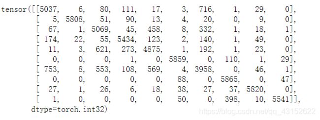
Lesson 28 CNN Confusion Matrix With PyTorch - Neural Network Programming

Confusion Matrix是一种可视化的工具，x轴代表的是预测种类，y轴代表的是真实种类，对应的二维坐标点是当某件物品的真实种类是y时，被认成x的个数，对角线上的数字表明对种类做出了正确的判断，其它的地方表明我们的model混淆了种类，所以这个矩阵被称为Confusion Matrix，
整理下构建Confusion Matrix的思路：
对于一个sample而言，我们会返回一个predict tensor，因为本次项目是一个10分类任务，所以tensor.Size为[1,10],通过argmax（dim=1）可以得到概率最高的那一个种类，这表示的是predict x，而真实有个label y，对应矩阵位置加1即可，我们得到所有的predict tensor以后就可以画出confusion matrix。这里有个细节是，在做前向传播做预测时，会生成动态计算图，但是为了节省性能我们不想要它，可以通过torch.no_grad()方法在局部禁用计算图。

@torch.no_grad()
def get_all_predict(train_loader,network):
	result = torch.tensor([],dtype=torch.int32)
	for batch in train_loader:
		images,labels = batch
		predict = network(images).argmax(dim=1)
		sample = torch.stack((labels,predict),dim=1)
		result = torch.cat((result,sample),dim=0)
	return result

定义了一个获得train_set中所有预测张量的函数,每次将一个批次进行前向传播，得到预测向量，然后利用argmax得到预测label，将真实label和预测label拼接，最后将所用结果沿一个新的轴堆叠。

train_loader = torch.utils.datasets(
	train_set,batch_size=1000
)
result = get_all_predict(train_loader,network)
result.require_grad
> False

cfm = torch.zeros((10,10),dtype=torch.int32)
for sample in result:
	rl,pl = sapmle.tolist()
	cfm[rl,pl] = cfm[rl,pl] + 1

下面进行绘制

import itertools
import numpy as np
import matplotlib.pyplot as plt

def plot_confusion_matrix(cm, classes, normalize=False, title='Confusion matrix', cmap=plt.cm.Blues):
    if normalize:
        cm = cm.astype('float') / cm.sum(axis=1)[:, np.newaxis]
        print("Normalized confusion matrix")
    else:
        print('Confusion matrix, without normalization')

    print(cm)
    plt.imshow(cm, interpolation='nearest', cmap=cmap)
    plt.title(title)
    plt.colorbar()
    tick_marks = np.arange(len(classes))
    plt.xticks(tick_marks, classes, rotation=45)
    plt.yticks(tick_marks, classes)

    fmt = '.2f' if normalize else 'd'
    thresh = cm.max() / 2.
    for i, j in itertools.product(range(cm.shape[0]), range(cm.shape[1])):
        plt.text(j, i, format(cm[i, j], fmt), horizontalalignment="center", color="white" if cm[i, j] > thresh else "black")

    plt.tight_layout()
    plt.ylabel('True label')
    plt.xlabel('Predicted label')

plt.figure(figsize=(10,10))
plot_confusion_matrix(confusion_matrix,train_set.classes)

Lesson 29 Stack Vs Concat In PyTorch,TensorFlow & Numpy - Deep Learning Tensors Ops

本章着重强调了tensor.stack和tensor.cat两个方法，cat是在现有轴进行拼接，stack要求两个tensor的shape必须一样，在一个新的轴上堆叠。
现在假设有3张单独的图片，它们都是3-d张量，如果想把它们合成一个batch，必须在一个新的batch轴上堆叠。
假设现在有一个batch的图片，又来了3张新的图片，新的图片无法和老的图片直接stack或者cat，可以把三张新的图片堆叠成一个batch，再把两个batch的数据进行堆叠。

Lesson 30 TensorBoard With PyTorch - Visualize Deep Learning Metrics

TensorBoard在机器学习中可以提供的可视化服务和工具：

1. 可视化和跟踪例如loss和arrcuracy的精度标准
2. 可视化计算图
3. 查看例如权重，偏置这些张量随着时间变化的柱状图
4. 展示图片，文字，或者语音数据

#查看tensorboard的版本
tensorboard --version
#安装tensorboard
pip install tensorboard

Tensorboard是一个前端页面接口，能够从文件里面读取数据并展示它。我们的任务之一就是将我们想让tensorboard展示的data存放进他能读取的文件中。
PyTorch创建了一个工具包来简化这个过程

from torch.utils.tensorboard import SummaryWriter

summary里面有许多的方法使得我们可以有选择性的将数据注入tensorboard中。

tb = SummaryWriter()
network = Network()
images,labels = next(iter(train_loader))
grid = torchvision.utils.make_grid(images)
tb.add_images('images',grid)
tb.add_gragh(network,images)
tb.close()

实例化了一个SummaryWriter的对象叫做tb，然后两个add方法就相当于把数据注入了tensorboard
启动Tensorboard，在控制台切换的当前工作目录，输入以下命令
tensorboard --logdir=runs
此时TensorBoard的服务器在localhost上开了一个端口6006.

tensorboard除了可以显示images和graph，还可以添加scalar和histogram。

tb.add_scalar('Accuracy',total_correct/len(train_set),epoch)
tb.add_scalar('Loss',total_loss,epoch)
tb.add_histogram('conv1.bias',network.conv1.bias,epoch)
tb.add_histogram('conv1.weight',network.conv1.weight,epoch)
tb.add_histogram('conv1.weight.grad',network.conv1.weight.grad,epoch)

Hyperparameter Tuning And Experimenting - Training Deep Neural Networks

使用TensorBoard来快速实验不同训练超参数的组合，它可以在改变超参数的时候来比较它们的结果。
为了发挥TensorBoard比较能力的优势，我们要运行多次实验，并且要唯一标识每次的running。
利用PyTorch提供的SummaryWriter这个类,一次运行会在对象实例被创建的时候开始，在实例被调用close方法时或者是离开作用域时结束。
为了唯一地标识每次运行，我们可以直接设置run下面的文件名称，或者是传递一个comment字符串到构造器里，然后这个comment string会被追加到这个自动生成的文件名称中。

# PyTorch version 1.1.0 SummaryWriter class
if not log_dir:
    import socket
    from datetime import datetime
    current_time = datetime.now().strftime('%b%d_%H-%M-%S')
    log_dir = os.path.join(
        'runs', 
        current_time + '_' + socket.gethostname() + comment
    )
self.log_dir = log_dir

我们每次在实例化Summary对象的时候并没有显式传入log_dir,所以利用的都是自动生成的，文件名称默认是time+host+comment,都在runs文件夹下。
下面开始尝试改变我们的超参数并且比较不同的实验结果。

batch_size = 100,
lr = 0.01
train_loader = torch.utils.data.DataLoader(
	train_set,batch_size = batch_size
)
optimizer = optim.Adam(network.parameters,lr=lr)
tb = SummaryWriter(comment=f'batch_size={batch_size} lr={lr}')

我们把以前那种硬编码的方法，改成了现在这种灵活的版本。在一个字符串前面加f的意思表示后面大括号里面要被解释成一个python表达式。

由于现在要考虑不同的batch_size,所以计算loss的方式要改变

#这是以前的代码
total += loss.item()
#这是现在的代码
total += loss.item() * batch_size

现在有个问题是，训练集可能不一定恰巧被batch平均分配，一种方法是在train_loader中设置一个参数叫drop_last，将其设置为True.如果不想丢弃最后一组数量不足的batch，那就使用每个batch第一个轴的长度代替batch_size

#第一种方法，丢弃最后一个batch
train_loader = torch.utils.data.DataLoader(
	train_set,batch_size=batch_size,drop_last=True
)
total_loss += loss.item() * batch_size
#第二种方法使用batch轴
total_loss += loss.item() * images.shape[0]

现在假设我们有两组超参数需要比较

batch_size_list = [10,100,1000]
lr_list = [0.01,0.001,0.0001]
for batch_size in batch_size_list:
	for lr in lr_list:
		network = Network()
		train_loader = torch.utils.data.DataLoader = (
			train_set,batch_size = batch_size
		)
		optimizer = optim.Adam(network.parameters(),lr=lr)
		comment=f'batch_size={batch_size} lr=={lr}'
		tb = SummaryWriter(comment=comment)

可以发现两组超参数就需要两个二嵌套循环，或者需要更多种类的超参数，那么就需要很多层嵌套循环。解决方法是使用笛卡尔积运算，可以得到所有超参数的组合，这样一个循环就能搞定。

from itertools import product
hyperparam = dict(
	lr:[.01,.001], 
	batch_size = [100,1000],
	shuffle = [True,False]
)
param_values = [v for v in hyperparam.values]
for lr,batch_size,shuffle in product(*param_values):
	print(lr,batch_size,shuffle)

for lr,batch_size,shuffle in product(*param_valus):
    train_loader = torch.utils.data.DataLoader(
        train_set,batch_size=batch_size,shuffle=shuffle
    )
    network = Network()
    optimizer = torch.optim.Adam(network.parameters(),lr=lr)
    tb = SummaryWriter(comment=f'batch_size={batch_size}lr={lr}shuffle={shuffle}')
    for epoch in range(10):
        total_loss = 0
        total_correct = 0
        for batch in train_loader:
            images,labels = batch
            predict = network(images)
            loss = F.cross_entropy(predict,labels)
            total_loss += loss.item() * images.shape[0]
            total_correct += get_correct_num(predict,labels)
            optimizer.zero_grad()
            loss.backward()
            optimizer.step()
            pass
        tb.add_scalar('Loss',total_loss,epoch)
        tb.add_scalar('Accuracy',total_correct/len(train_set),epoch)
        for name,weight in network.named_parameters():
            tb.add_histogram(name,weight,epoch)
            tb.add_histogram(f'{name}.grad',weight.grad,epoch)
        print(
            'epoch',epoch,
            'loss',total_loss,
            'accuracy',total_correct / len(train_set)
        )

Lesson 32 Training Loop Run Builder - Neural Network Experimentation Code

本节的目的是使得我们在训练过程中高效的进行实验。因此想要将上一节的超参数实验变得更整洁。

class RunBuilder():
	@staticmethod
	def get_runs(params):
		Run = namedtuple('Run',params.keys())
		runs = []
		for v in product(*params.values()):
			runs.append(Run(*v))
		return runs

这个类的作用就是通过传入一个参数来定制化我们的run。

params = OrderedDict(
	lr = [.01,.001],
	batch_size=[1000,10000]
)

we want to do a training run for each learning rate and each batch size in the dictoinary。

runs = RunBuilder.get_runs(params)
runs
[
	Run(lr=0.01,batch_size=1000),
	Run(lr=0.01,batch_size=10000),
	Run(lr=0.001, batch_size=1000),
    Run(lr=0.001, batch_size=10000)
]

这个list里面包含了4个string表达式，这使得我们可以唯一标识一个run，而且还可以通过run.lr,run.batch_size拿到里面的每个超参数.
OrderedDic与普通dict的区别是它里面的属性是有顺序的，保证顺序可以使得后面的key和values不会对应错。
namedtuple（typename,keys）
可以返回一个创造具名元组的类，typename就是给一个类取个名字，keys就是为元组中的每一个位置上的value起一个名字。

Lesson 33 CNN Training Loop Refactoring - Simultaneous Hyperparameter Testing

本节的目的是当有大量的超参数的时候，我们仍然可以使得我们的训练循环和结果变得有序。首先我们需要的第一个类是RunBuilder

class RunBuilder():
	@static_method
	def get_runs(params):
		Run = namedtuple('Run',params.key())
		runs = []
		for v in product(*params.values()):
			runs.append(Run(*v))
		return runs

这样既可以得到定制化的run

for run in RunBuilder.get_runs(params):

接下来我们会创建一个RunManager的类，它将使得我们能够在每一个run中进行管理，一方面可以摆脱(pull out)冗长的TensorBoard调用，另一方面可以增加一些其他的功能。当parameter和run的数量增多的时候，TensorBoard不再是一个可以查看结果的可行方案。
RunManager将在每个执行过程中创建生命周期，还可以跟踪损失和正确的预测数，最终还可以将运行结果保存到磁盘上。

class RunManager():
	def __init__(self):
		self.epoch_count = 0 #the number of epochs
		self.epoch_loss = 0 #The running loss for an epoch
		self.epoch_num_correct = 0 #The number of correct predictions for an epoch
		self.epoch_start_time = None#The start time of an epoch
		self.run_params = None #one of the run returned by the RunBuilder
		self.run_count = 0
		self.run_data = []
		self.run_start_time = None
		self.network = None
		self.loader = None
		self.tb = None

博文中提出了一个很有意思的词，叫做code smell，有什么地方觉得让人不舒服。比如那些属性前面都有相同的前缀，本就应该在一起，所以用面向对象的思想来解决这个。

class Epoch():
	def __init__(self):
		self.count = 0
		self.loss = 0
		self.num_correct = 0
		self.start_time = None

class RunManager():
    def __init__(self):
        self.start_time = None
        self.run_params = None
        self.run_count = 0
        self.run_data = []

        self.network = None
        self.loader = None
        self.tb = None

        self.epoch_start_time = None
        self.epoch_count = 0
        self.epoch_loss = 0
        self.epoch_num_correct = 0

    def get_correct_num(self,predict, labels):
        return predict.argmax(dim=1).eq(labels).sum().item()

    def begin_run(self, run,network, loader):
        self.run_params = run
        self.start_time = time.time()
        self.run_count += 1
        self.tb = SummaryWriter(comment=f'{run}')
        self.network = network
        self.loader = loader
        images, labels = next(iter(loader))
        self.tb.add_images('images', images)
        self.tb.add_graph(network, images)

    def begin_epoch(self):
        self.epoch_count += 1
        self.epoch_start_time = time.time()
        self.epoch_num_correct = 0
        self.epoch_loss = 0
        pass

    def end_epoch(self):
        epoch_duration = time.time() - self.epoch_start_time
        run_duration = time.time() - self.start_time
        loss = self.epoch_loss / len(self.loader.dataset)
        accuracy = self.epoch_num_correct/len(self.loader.dataset)
        self.tb.add_scalar('Loss', loss, self.epoch_count)
        self.tb.add_scalar('Accuracy', accuracy, self.epoch_count)
        for name, weight in self.network.named_parameters():
            self.tb.add_histogram(name, weight, self.epoch_count)
            self.tb.add_histogram(f'{name}.grad', weight.grad, self.epoch_count)
            pass
        results = OrderedDict(
            run=self.run_count,
            epoch=self.epoch_count,
            loss=loss,
            accuracy=accuracy,
            epoch_duration=epoch_duration,
            run_duration=run_duration
        )
        for k, v in self.run_params._asdict().items():results[k] = v
        self.run_data.append(results)
        df = pd.DataFrame.from_dict(self.run_data, orient='columns')
        clear_output(wait=True)
        display(df)
        pass

    def track_loss(self, loss,batch):
        self.epoch_loss += loss.item() * batch[0].shape[0]
        pass

    def track_num_correct(self, preds, labels):
        self.epoch_num_correct += self.get_correct_num(preds, labels)

    def end_run(self):
        self.tb.close()
        self.epoch_count = 0

for run in RunBuilder.get_runs(params):
    network = Network()
    train_loader = torch.utils.data.DataLoader(
        train_set,batch_size=run.batch_size
    )
    optimizer = optim.Adam(network.parameters(),lr=run.lr)
    manager.begin_run(run=run,network=network,loader=train_loader)
    for epoch in range(5):
        manager.begin_epoch()        
        for batch in train_loader:
            images, labels = batch
            predict = network(images)
            loss = F.cross_entropy(predict,labels)
            manager.track_loss(loss,batch)
            manager.track_num_correct(preds=predict,labels=labels)
            optimizer.zero_grad()
            loss.backward()
            optimizer.step()
            pass
        manager.end_epoch()
    manager.end_run()
  

Lesson 34 PyTorch DataLoader Num_workers - Deep Learning Speed Limit Increase

本节教我们使用了DataLoader多进程加载训练数据的方法，DataLoader有一个num_workers的属性，默认是0，表示只使用主进程加载batch，然而可以多开几个进程，这样同时可以加载多个batch的数据，num_workers不是越多越好，当前向传播和后向传递所消耗的时间大于一个batch的数据加载时间，那么把num-workers设置为1就足够了。

Lesson 35 PyTorch Code On A GPU - Neural NetworkProgramming Guide

PyTorch允许我们在GPU和CPU之间实现数据的无缝转移，当我们想要把数据转去GPU时，我们使用cuda，当我们使用CPU时，我们使用cpu，还有to这个方法使用。当要把数据转向GPU时我们使用to(‘cuda’)，当我们使用cpu时，我们使用to(‘cpu’).
要想在训练过程中使用GPU，必须将data和network都转移向GPU，但是，当tensor和network创建的时候，data都在CPU的内存中。

t = torch.ones(1,1,28,28)
network = Network()
t = t.cuda()
network = network.cuda()

注意，数据与数据之间，数据与网络之间它们必须在一个设备上。说是网络在设备上其实不准确，网络其实是由其中的张量和transformation来决定的，所以其实还是张量在设备上。

我们在编写代码的时候并不知道代码运行在什么样的设备上，这被称为Device Agnostic，所以cuda和cpu这种硬编码的代码不太常用，而to这个方法可以通过传参数来决定使用什么设备。
torch.cuda.is_avaliable()根据返回结果给参数字符串赋值。

Lesson 36 PyTorch Dataset Normalization - Torchvision.Transforms.Normalize()

Normalization 也叫 feature scaling。这个术语的出现是因为当我们在normalizing数据的时候，我们经常会将不同的feature转换成相似的形状。

Data standardization 是一种特殊的normalization工具，也可以叫做z-score normalization
$z=\frac{x-mean}{std}$
mean是当前数据集合的均值，std是当前集合的方差
以下是实现Normalize的方法，首先得得到各个feature的mean和std
有两种方法，分别是一种简单的方法和一种困难的方法。当我们的数据集比较小的时候，可以使用简单的方法，当数据集比较大内存一次装不下的时候就需要使用困难的就需要使用困难的方法。

loader = DataLoader(train_set,batch_size=len(train_set),num_workers=1)
data = netxt(iter(loader))
data[0].mean(),data[0].std()

#先计算总共的像素点个数
num_of_pixels = len(train_set) * 28 * 28 #样本数乘以宽和高
total_sum = 0
for batch in train_loader:total_sum += batch[0].sum
mean = total_sum / num_of_pixes
sum_of_squard_error = 0
for batch in train_loader:
	sum_of_squard_error += ((batch[0] - mean).pow(2)).sum()
std = torch.sqrt(sum_of_squared_error / num_of_pixes)

下面根据std和mean来构造一个新的train_set

train_set = tochvision.datasets.FashionMNIST(
	root='./data',
	download=True,
	train=True,
	transform=transform.Compos(
		[
			transforms.ToTensor(),
			transforms.Nomalize(mean,std)
		]
	)
)

如果我们有RGB三个颜色通道的话就需要分别计算三个通道的mean和std
transforms.Normalize(
[meanofchannel1,meanofchannel2,meanofchannel3],
[stdofchannel1,stdofchannel2,stdofchannel3]
)
注意一点Totensor必须在Normalize之前

Lesson 37 PyTorch DataLoader Source Code - Debugging Session

to see the video in Bilibili