涡扇发动机的预测性维护

探索NASA的涡扇数据集 (Exploring NASA’s turbofan dataset)

Although released over a decade ago, NASA’s turbofan engine degradation simulation dataset (CMAPSS) remains popular and relevant today. Over 90 new research papers have been published in 2020 so far [1]. These papers present and benchmark novel algorithms to predict Remaining Useful Life (RUL) on the turbofan datasets.

尽管已经发布了十多年，但NASA的涡扇发动机退化模拟数据集(CMAPSS)仍然很受欢迎，并在今天具有重要意义。 截止到2020年，已有90多篇新研究论文发表[1]。 这些论文提出了新的算法并对其进行了基准测试，以预测涡轮风扇数据集上的剩余使用寿命(RUL)。

When I first started learning about predictive maintenance, I stumbled upon a few blog posts using the turbofan degradation dataset. Each covered exploratory data analysis and a simple model to predict the RUL, but I felt two things were lacking:

当我第一次开始学习预测性维护时，我偶然发现了一些使用涡轮风扇降级数据集的博客文章。 每个都包含探索性数据分析和一个简单的模型来预测RUL，但是我感到缺少两件事：

1. I never got a complete overview of how to apply different suitable techniques to the same problem
   对于如何将不同的适用技术应用于同一问题，我从未获得完整的概述。
2. The blog posts would only focus on the first dataset, leaving me guessing how the more complex challenges could be solved.
   博客文章仅关注第一个数据集，让我猜测如何解决更复杂的挑战。

A few years later this seemed like a fun project for me to pick up. In a series of posts, I plan to showcase and explain multiple analysis techniques, while also offering a solution for the more complex datasets.

几年后，这对我来说似乎是一个有趣的项目。 在一系列文章中，我计划展示和解释多种分析技术，同时还为更复杂的数据集提供解决方案。

I’ve created an index below which I’ll update with links to new posts along the way:

我创建了一个索引，在该索引下，我将通过以下方式更新指向新帖子的链接：

1. FD001 — Exploratory data analysis and baseline model (this article) 2. FD001 — Updated assumption of RUL & Support Vector Regression 3. FD001 — Time series analysis: distributed lag models4. FD001 — Survival analysis for predictive maintenance5. FD003 — Random forest (I’ve changed the order, read the article to find out why) 6. FD002 — lagged MLP & reproducible results primer 7. FD004 — LSTM & wrap-up

1. FD001-探索性数据分析和基线模型(本文)2. FD001-RUL和支持向量回归的更新假设3. FD001-时间序列分析：分布式滞后模型4。 FD001 —预测性维护的生存分析5。 FD003 —随机森林(我更改了顺序，阅读文章以找出原因)6. FD002 —落后的MLP和可再现的结果引物7. FD004 — LSTM和总结

The turbofan dataset features four datasets of increasing complexity (see table I) [2, 3]. The engines operate normally in the beginning but develop a fault over time. For the training sets, the engines are run to failure, while in the test sets the time series end ‘sometime’ before failure. The goal is to predict the Remaining Useful Life (RUL) of each turbofan engine.

涡轮风扇数据集具有四个复杂度不断提高的数据集(请参见表I)[2，3]。 发动机在一开始就正常运行，但随着时间的流逝会出现故障。 对于训练集，引擎将运行至故障，而在测试集中，时间序列将在故障发生之前的“某个时候”结束。 目的是预测每个涡轮风扇发动机的剩余使用寿命(RUL)。

Table I: Overview of turbofan datasets 表一：涡轮风扇数据集概述

Datasets include simulations of multiple turbofan engines over time, each row contains the following information: 1. Engine unit number 2. Time, in cycles 3. Three operational settings 4. 21 sensor readings

数据集包括随时间变化的多个涡轮风扇发动机的仿真，每一行包含以下信息：1.发动机单元编号2.周期时间3.三种运行设置4. 21个传感器读数

What I find really cool about this dataset is that you can’t use any domain knowledge, as you don’t know what a sensor has been measuring. So, results are purely based on applying the correct techniques.

我发现此数据集的真正酷点是您不能使用任何领域知识，因为您不知道传感器正在测量什么。 因此，结果完全基于应用正确的技术。

In today’s post we’ll focus on exploring the first dataset (FD001) in which all engines develop the same fault and have only one operating condition. In addition, we’ll create a baseline linear regression model so we can compare our modeling efforts of future posts.

在今天的帖子中，我们将重点研究第一个数据集(FD001)，在该数据集中，所有引擎都出现相同的故障，并且只有一个工作状态。 另外，我们将创建一个基线线性回归模型，以便我们可以比较未来职位的建模工作。

探索性数据分析 (Exploratory Data Analysis)

Let’s get started by importing the required libraries, read the data and inspect the first few rows. Note that a few columns seem to have none to very little deviation in their values. We’ll explore these further down below.

首先，导入所需的库，读取数据并检查前几行。 请注意，几列的值似乎没有或几乎没有偏差。 我们将在下面进一步探讨这些内容。

%matplotlib inline
import pandas as pd
import numpy as np
import matplotlib.pyplot as plt
import seaborn as sns; sns.set()


from sklearn.linear_model import LinearRegression
from sklearn.metrics import mean_squared_error, r2_score

# define filepath to read data
dir_path = './CMAPSSData/'


# define column names for easy indexing
index_names = ['unit_nr', 'time_cycles']
setting_names = ['setting_1', 'setting_2', 'setting_3']
sensor_names = ['s_{}'.format(i) for i in range(1,22)] 
col_names = index_names + setting_names + sensor_names


# read data
train = pd.read_csv((dir_path+'train_FD001.txt'), sep='\s+', header=None, names=col_names)
test = pd.read_csv((dir_path+'test_FD001.txt'), sep='\s+', header=None, names=col_names)
y_test = pd.read_csv((dir_path+'RUL_FD001.txt'), sep='\s+', header=None, names=['RUL'])


# inspect first few rows
train.head()

Result of train.head() train.head()的结果

Next, FD001 should contain data of one hundred engines, let’s inspect the unit number to verify this is the case. I chose to use pandas describe function so we can also get an understanding of the distribution. While we’re at it, let’s also inspect the time cycles to see what we can learn about the number of cycles the engines ran on average before breaking down.

接下来，FD001应该包含一百个引擎的数据，让我们检查单元号以验证是否是这种情况。 我选择使用pandas describe函数，以便我们也可以了解其分布。 在此过程中，我们还要检查时间周期，以了解有关发动机在发生故障之前平均运行的周期数的信息。

train[index_names].describe()
train[index_names].groupby('unit_nr').max().describe()

Dataset descriptive statistics of unit_nr and time_cycles unit_nr和time_cycles的数据集描述性统计

When we inspect the descriptive statistics of unit_nr we can see the dataset has a total of 20631 rows, unit numbers start at 1 and end at 100 as expected. What’s interesting, is that the mean and quantiles don’t align neatly with the descriptive statistics of a vector from 1–100, this can be explained due to each unit having different max time_cycles and thus a different number of rows. When inspecting the max time_cycles you can see the engine which failed the earliest did so after 128 cycles, whereas the engine which operated the longest broke down after 362 cycles. The average engine breaks between 199 and 206 cycles, however the standard deviation of 46 cycles is rather big. We’ll visualize this further down below to get an even better understanding.

当我们检查unit_nr的描述性统计信息时，我们可以看到数据集共有20631行，单元号按预期从1开始到100结束。 有趣的是，均值和分位数与从1到100的向量的描述统计数据不一致，这可以解释，因为每个单元具有不同的max time_cycles，因此行数不同。 检查最大time_cycles时，您可以看到最早失效的发动机是在128个循环后失效的，而运行时间最长的发动机则在362个循环后发生了故障。 平均发动机在199和206周期之间断裂，但是46周期的标准偏差相当大。 我们将在下面进一步可视化此内容，以更好地理解。

The dataset description also indicates the turbofans run at a single operating condition. Let’s check the settings for verification.

数据集描述还指示涡轮风扇在单个运行条件下运行。 让我们检查设置以进行验证。

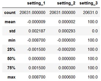
train[setting_names].describe()

Descriptive statistics of engine settings 引擎设置的描述性统计

Looking at the standard deviations of settings 1 and 2, they aren’t completely stable. The fluctuations are so small however, that no other operating conditions can be identified.

查看设置1和2的标准偏差，它们并不完全稳定。 但是，波动很小，无法确定其他运行条件。

Finally, we’ll inspect the descriptive statistics of the sensor data, looking for indicators of signal fluctuation (or the absence thereof).

最后，我们将检查传感器数据的描述性统计信息，寻找信号波动(或不存在)的指标。

train[sensor_names].describe().transpose()

Descriptive statistics of the sensor signals. 传感器信号的描述性统计。

By looking at the standard deviation it’s clear sensors 1, 10, 18 and 19 do not fluctuate at all, these can be safely discarded as they hold no useful information. Inspecting the quantiles indicates sensors 5, 6 and 16 have little fluctuation and require further inspection. Sensors 9 and 14 have the highest fluctuation, however this does not mean the other sensors can’t hold valuable information.

通过查看标准偏差，可以清楚地看出传感器1、10、18和19根本没有波动，由于它们没有任何有用的信息，因此可以安全地丢弃它们。 检查分位数表明传感器5、6和16的波动很小，需要进一步检查。 传感器9和14的波动最大，但这并不意味着其他传感器无法保存有价值的信息。

计算RUL (Computing RUL)

Before we start plotting our data to continue our EDA, we’ll compute a target variable for Remaining Useful Life (RUL). The target variable will serve two purposes:

在开始绘制数据以继续执行EDA之前，我们将计算“剩余使用寿命”(RUL)的目标变量。 目标变量将用于两个目的：

1. It will serve as our X-axis while plotting sensor signals, allowing us to easily interpret changes in the sensor signals as the engines near breakdown.
   在绘制传感器信号时，它将用作我们的X轴，使我们可以轻松地解释当发动机接近故障时传感器信号的变化。
2. It will serve as target variable for our supervised machine learning models.
   它将用作我们监督的机器学习模型的目标变量。

Without further information about the RUL of engines in the training set, we’ll have to come up with estimates of our own. We’ll assume the RUL decreases linearly over time and have a value of 0 at the last time cycle of the engine. This assumption implies RUL would be 10 at 10 cycles before breakdown, 50 at 50 cycles before breakdown, etc.

如果在培训集中没有关于引擎RUL的进一步信息，我们将不得不对自己的估计。 我们假设RUL随时间线性下降，并且在引擎的最后一个时间周期的值为0。 此假设意味着RUL在击穿前10个周期为10，在击穿前50个周期为50，依此类推。

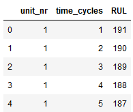
Mathematically we can use max_time_cycle — time_cycle to compute our desired RUL. Since we want to take the max_time_cycle of each engine into account, we’ll group the dataframe by unit_nr before computing max_time_cycle. The max_time_cycle is then merged back into the dataframe to allow easy calculation of RUL by subtracting the columns max_time_cycle — time_cycle. Afterwards we drop max_time_cycle as it’s no longer needed and inspect the first few rows to verify our RUL calculation.

在数学上，我们可以使用max_time_cycle — time_cycle计算所需的RUL。 由于我们要考虑每个引擎的max_time_cycle ， unit_nr在计算max_time_cycle之前，将数据帧按unit_nr max_time_cycle 。 然后，将max_time_cycle合并回数据帧，以通过减去max_time_cycle — time_cycle列轻松地计算RUL。 然后，我们删除不再需要的max_time_cycle并检查前几行以验证我们的RUL计算。

def add_remaining_useful_life(df):
    # Get the total number of cycles for each unit
    grouped_by_unit = df.groupby(by="unit_nr")
    max_cycle = grouped_by_unit["time_cycles"].max()
    
    # Merge the max cycle back into the original frame
    result_frame = df.merge(max_cycle.to_frame(name='max_cycle'), left_on='unit_nr', right_index=True)
    
    # Calculate remaining useful life for each row
    remaining_useful_life = result_frame["max_cycle"] - result_frame["time_cycles"]
    result_frame["RUL"] = remaining_useful_life
    
    # drop max_cycle as it's no longer needed
    result_frame = result_frame.drop("max_cycle", axis=1)
    return result_frame
  
train = add_remaining_useful_life(train)
train[index_names+['RUL']].head()

绘图 (Plotting)

Plotting is always a good idea to develop a better understanding of your dataset. Let’s start by plotting the histogram of max RUL to understand its distribution.

绘图始终是一个更好的了解数据集的好主意。 让我们首先绘制最大RUL的直方图以了解其分布。

df_max_rul = train[['unit_nr', 'RUL']].groupby('unit_nr').max().reset_index()
df_max_rul['RUL'].hist(bins=15, figsize=(15,7))
plt.xlabel('RUL')
plt.ylabel('frequency')
plt.show()

The histogram reconfirms most engines break down around 200 cycles. Furthermore, the distribution is right skewed, with few engines lasting over 300 cycles.

直方图可以确认大多数引擎在200个循环左右时就崩溃了。 此外，该分布是右偏的，几乎没有引擎能够持续300个循环。

Below I’ll show the code used to plot signals of each sensor. Due to the large number of engines, it’s not feasible to plot every engine for every sensor. The graphs would no longer be interpret-able with so many lines in one plot. Therefore, I chose to plot each engine whose unit_nr is divisible by 10 with a remainder of 0. We revert the X-axis so RUL decreases along the axis, with a RUL of zero indicating engine failure. Due to the large number of sensors I’ll discuss a few graphs which are representative for the whole set. Remember, based on our descriptive statistics, we should definitely inspect the graphs of sensors 5, 6 and 16.

下面，我将显示用于绘制每个传感器信号的代码。 由于引擎数量众多，因此无法为每个传感器绘制每个引擎。 一张图中的这么多线将无法解释这些图。 因此，我选择绘制每个unit_nr被10整除且余数为0的引擎的图。我们还原X轴，以使RUL沿该轴减小，RUL为零表示引擎故障。 由于传感器数量众多，我将讨论一些代表整个集合的图表。 请记住，基于我们的描述性统计数据，我们绝对应该检查传感器5、6和16的图形。

def plot_sensor(sensor_name):
    plt.figure(figsize=(13,5))
    for i in train['unit_nr'].unique():
        if (i % 10 == 0):  # only plot every 10th unit_nr
            plt.plot('RUL', sensor_name, 
                     data=train[train['unit_nr']==i])
    plt.xlim(250, 0)  # reverse the x-axis so RUL counts down to zero
    plt.xticks(np.arange(0, 275, 25))
    plt.ylabel(sensor_name)
    plt.xlabel('Remaining Use fulLife')
    plt.show()

for sensor_name in sensor_names:
    plot_sensor(sensor_name)

Graph of s_1 vs declining RUL s_1与RUL下降的图表

The graph of sensors 1, 10, 18 and 19 look similar, the flat line indicates the sensors hold no useful information, which reconfirms our conclusion from the descriptive statistics. Sensors 5 and 16 also show a flat line, these can be added to the list of sensors to exclude.

传感器1、10、18和19的图形看起来相似，实线表示传感器没有任何有用的信息，这再次证实了我们从描述性统计中得出的结论。 传感器5和16也显示一条平线，可以将其添加到要排除的传感器列表中。

Graph of s_2 vs declining RUL s_2与下降RUL的关系图

Sensor 2 shows a rising trend, a similar pattern can be seen for sensors 3, 4, 8, 11, 13, 15 and 17.

传感器2呈上升趋势，对于传感器3、4、8、11、13、15和17可以看到类似的模式。

Graph of s_6 vs declining RUL s_6与RUL下降的图表

Sensor readings of sensor 6 peak downwards at times but there doesn’t seem to be a clear relation to the decreasing RUL.

传感器6的传感器读数有时会向下峰值，但似乎与RUL的下降没有明显关系。

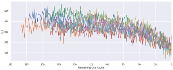
Graph of s_7 vs RUL s_7和RUL的图表

Sensor 7 shows a declining trend, which can also be seen in sensors 12, 20 and 21.

传感器7呈下降趋势，这在传感器12、20和21中也可以看到。

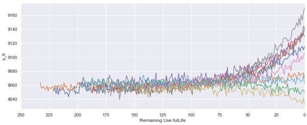
Graph of s_9 vs RUL s_9和RUL的图表

Sensor 9 has a similar pattern as sensor 14.

传感器9具有与传感器14类似的样式。

Based on our Exploratory Data Analysis we can determine sensors 1, 5, 6, 10, 16, 18 and 19 hold no information related to RUL as the sensor values remain constant throughout time. Let’s kick-off our model development with a baseline Linear Regression model. The model will use the remaining sensors as predictors.

根据我们的探索性数据分析，我们可以确定传感器1、5、6、10、16、18和19没有保存与RUL相关的信息，因为传感器值在整个时间内保持恒定。 让我们从基线线性回归模型开始我们的模型开发。 该模型将使用其余的传感器作为预测变量。

基线线性回归 (Baseline Linear Regression)

First, we’ll define a small function to evaluate our models. I chose to include Root Mean Squared Error (RMSE) as it will give an indication how many time cycles the predictions are off on average, and Explained Variance (or R² score) to indicate what proportion of our dependent variable can be explained by the independent variables we use.

首先，我们将定义一个小的函数来评估我们的模型。 我选择包括均方根误差(RMSE)，因为它可以表明预测平均偏离了多少个时间周期，而解释方差(或R²得分)则表明我们独立变量可以解释我们的因变量的比例我们使用的变量。

def evaluate(y_true, y_hat, label='test'):
    mse = mean_squared_error(y_true, y_hat)
    rmse = np.sqrt(mse)
    variance = r2_score(y_true, y_hat)
    print('{} set RMSE:{}, R2:{}'.format(label, rmse, variance))

We’ll drop the unit_nr, time_cycle, settings and sensors which hold no information. The RUL column of the training set is stored in its own variable. For our test set we drop the same columns. In addition, we are only interested in the last time cycle of each engine in the test set as we only have True RUL values for those records.

我们将删除不unit_nr, time_cycle, settings and sensors任何信息的unit_nr, time_cycle, settings and sensors 。 训练集的RUL列存储在其自己的变量中。 对于我们的测试集，我们删除相同的列。 此外，我们只对测试集中每个引擎的最后一个时间周期感兴趣，因为我们只有那些记录的True RUL值。

drop_sensors = ['s_1','s_5','s_6','s_10','s_16','s_18','s_19']
drop_labels = index_names+setting_names+drop_sensors


X_train = train.drop(drop_labels, axis=1)
y_train = X_train.pop('RUL')


# Since the true RUL values for the test set are only provided for the last time cycle of each enginge, 
# the test set is subsetted to represent the same
X_test = test.groupby('unit_nr').last().reset_index().drop(drop_labels, axis=1)

Setting up for linear regression is quite straightforward. We instantiate the model by simply calling the method and assigning it to the ‘lm’ variable. Next, we fit the model by passing our ‘X_train’ and ‘y_train’. Finally, we predict on both the train and test set to get the full picture of how our model is behaving with the data that was presented to it.

设置线性回归非常简单。 我们通过简单地调用方法并将其分配给“ lm”变量来实例化模型。 接下来，我们通过传递“ X_train”和“ y_train”来拟合模型。 最后，我们在训练集和测试集上进行预测，以全面了解我们的模型如何利用提供给它的数据来表现。

# create and fit model
lm = LinearRegression()
lm.fit(X_train, y_train)


# predict and evaluate
y_hat_train = lm.predict(X_train)
evaluate(y_train, y_hat_train, 'train')


y_hat_test = lm.predict(X_test)
evaluate(y_test, y_hat_test)

# returns
# train set RMSE:44.66819159545453, R2:0.5794486527796716
# test set RMSE:31.952633027741815, R2:0.40877368076574083

Note, the RMSE is lower on the test set, which is counter-intuitive, as commonly a model performs better on the data it has seen during training.

注意，RMSE在测试集上较低，这是违反直觉的，因为通常模型在训练过程中看到的数据表现更好。

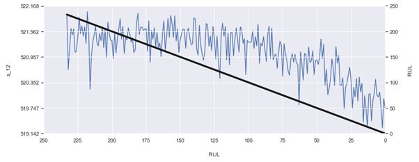
A possible explanation could be the computed RUL of the training set ranging well into the 300s. Looking at the trend of the graph below, the higher values of linearly computed RUL do not seem to correlate very well with the sensor signal. Since RUL predictions of the test set are closer to failure, and the correlation between the lower target RUL and sensor signal is clearer, it may be easier for the model to make accurate predictions on the test set. The large difference in train and test RMSE can be seen as a flaw of our assumption of RUL and is something we’ll try to improve in the future. For now, we have concluded our EDA and baseline model.

一个可能的解释可能是训练集的计算RUL范围一直到300 s。 查看下图的趋势，线性计算的RUL的较高值似乎与传感器信号没有很好的相关性。 由于测试集的RUL预测更接近故障，并且较低的目标RUL和传感器信号之间的相关性更加清晰，因此模型可能更容易在测试集上做出准确的预测。 训练和测试RMSE的巨大差异可以看作是我们对RUL的假设的缺陷，并且是我们将来会尝试改进的东西。 目前，我们已经结束了我们的EDA和基线模型。

Graph depicting linear declining RUL and s_12. This graph aims to showcase where the sensor signal and linearly declining RUL correlate strongly. 该图描述了线性下降的RUL和s_12。 该图旨在展示传感器信号和线性下降的RUL强烈相关的地方。

In today’s post we explored the first dataset of NASA’s turbofan degradation simulation dataset and created a baseline model with a test RMSE of 31.95. I would like to thank Maikel Grobbe and Wisse Smit for their inputs and reviewing my article. In the next post we’ll look at how to improve the computed RUL to make predictions more accurate. In addition, we’ll develop a Support Vector Regression to push performance even further.

在今天的帖子中，我们探索了NASA涡扇退化模拟数据集的第一个数据集，并创建了测试RMSE为31.95的基线模型。 我要感谢Maikel Grobbe和Wisse Smit的投入并审阅了我的文章。 在下一篇文章中，我们将研究如何改进计算的RUL以使预测更加准确。 此外，我们将开发支持向量回归以进一步提高性能。

If you have any questions or remarks, please leave them in the comments below. For the complete notebook you can check out my github page here.

如果您有任何疑问或意见，请留在下面的评论中。 对于完整的笔记本，您可以在这里查看我的github页面。

References:[1] Papers published on NASA’s CMAPSS data in 2020 so far: Google scholar search, accessed on 2020–08–08[2] A. Saxena, K. Goebel, D. Simon, and N. Eklund, “Damage Propagation Modeling for Aircraft Engine Run-to-Failure Simulation”, in the Proceedings of the Ist International Conference on Prognostics and Health Management (PHM08), Denver CO, Oct 2008.[3] NASA’s official data repository

参考文献：[1]到目前为止，有关2020年NASA的CMAPSS数据的论文： Google学术搜索 ，于2020-08-08年访问[2] A. Saxena，K。Goebel，D.Simon和N. Eklund，“损害传播”飞机发动机失效仿真模型”，在第一届国际预测与健康管理会议(PHM08)上，美国丹佛市，2008年10月。[3] NASA的官方数据存储库

翻译自: https://towardsdatascience.com/predictive-maintenance-of-turbofan-engines-ec54a083127