【mmdetection】RetinaNet解析 以RetinaNet为例 解析目标检测中的anchor生成、匹配、编解码策略

1. RetinaNet

one-stage detector

• 创新点：RetinaNet网络+Focal loss解决正负样本不平衡
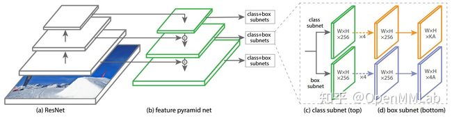
• 结构：backbone + fpn + head (bbox & class)
  

2. 配置文件

retinanet_r50_fpn.py解析如下：

backbone

• 配置

model = dict(
    type='RetinaNet',   # model名称
    backbone=dict(
        type='ResNet',   # backbone名称，采用ResNet
        depth=50,		# ResNet 50
        num_stages=4,	# ResNet设计范式为 stem + 4_stage，4就表示采用的stage的数量
        out_indices=(0, 1, 2, 3),   # backbone输出了4张特征图，索引分别为(0,1,2,3)，stride分别为(4,8,16,32)，输出通道数分别为(256,512,1024,2048)
        frozen_stages=1,	# 表示冻结stem和第一个stage的权重，不训练
        norm_cfg=dict(type='BN', requires_grad=True), # 是否需要进行参数更新
        norm_eval=True,	# 整个backbone网络的归一化算子变成eval模式，均值和方差采用预训练值，不更新。
        # norm_eval控制整个backbone的归一化算子是否需要变成eval模式
        style='pytorch',
        init_cfg=dict(type='Pretrained', checkpoint='torchvision://resnet50')), 
        # backbone采用pytorch提供的在imagenet上的预训练权重

out_indices： 一般分类模型都遵循 stem + n_stage + fc_head 的结构，ResNet为 stem+4stage+fc 3个部分。stem输出的stride为4，4个stage的stride分别为4,8,16,32，如 out_indices=(0,) 表示输出stride为4的特征图。backbone后接FPN，需4个feature map。
frozen_stages=-1（不冻结），0(stem)，1(stem+stage1)，2(stem+stage1+stage2)
参看mmdet/models/backbones/resnet.py，可以看到resnet的构建。
复习卷积/池化的feature map尺寸计算：$W^{\prime }=\frac{W-F+2P}{S}+1$；空洞卷积$W^{\prime }=\frac{W-d(F-1)-1+2P}{S}+1$。（向下取整）实际卷积核大小相当于$d(F-1)+1$，d为空洞率，在卷积核之间填充(d-1)个0。

1. stem：相较于原图的stride=4，输出通道数=64。stem由：conv(+norm+relu)+maxpool构成（依据conv+norm+relu的数量为1还是3，分为stem和deep_stem）。feature map 的尺寸经过conv+maxpool之后缩小了4倍，即stem的stride为4。

    def _make_stem_layer(self, in_channels, stem_channels):
        if self.deep_stem:    # conv + norm + relu + maxpool
            self.stem = nn.Sequential(
                build_conv_layer(
                    self.conv_cfg,
                    in_channels,
                    stem_channels // 2,
                    kernel_size=3,
                    stride=2,
                    padding=1,
                    bias=False),
                build_norm_layer(self.norm_cfg, stem_channels // 2)[1],
                nn.ReLU(inplace=True),
                build_conv_layer(
                    self.conv_cfg,
                    stem_channels // 2,
                    stem_channels // 2,
                    kernel_size=3,
                    stride=1,
                    padding=1,
                    bias=False),
                build_norm_layer(self.norm_cfg, stem_channels // 2)[1],
                nn.ReLU(inplace=True),
                build_conv_layer(
                    self.conv_cfg,
                    stem_channels // 2,
                    stem_channels,
                    kernel_size=3,
                    stride=1,
                    padding=1,
                    bias=False),
                build_norm_layer(self.norm_cfg, stem_channels)[1],
                nn.ReLU(inplace=True))
        else:
            self.conv1 = build_conv_layer(
                self.conv_cfg,
                in_channels,
                stem_channels,
                kernel_size=7,
                stride=2,
                padding=3,
                bias=False)
            self.norm1_name, norm1 = build_norm_layer(
                self.norm_cfg, stem_channels, postfix=1)
            self.add_module(self.norm1_name, norm1)
            self.relu = nn.ReLU(inplace=True)
        self.maxpool = nn.MaxPool2d(kernel_size=3, stride=2, padding=1)

2. stage：stride=(1,2,2,2)，即经过每个stage，feature map缩小的倍数，相较于原图缩小的倍数分别为4,8,16,32，通道数分别为256,512,1024,2048。构建细节这里不再赘述。
3. ResNet的前向过程：只有在 self.out_indices 中的feature map才输出，这里4个stage的feature map全部输出作为后面neck的输入。

   def forward(self, x):
        """Forward function."""
        if self.deep_stem:
            x = self.stem(x)
        else:
            x = self.conv1(x)
            x = self.norm1(x)
            x = self.relu(x)
        x = self.maxpool(x)
        outs = []
        for i, layer_name in enumerate(self.res_layers):
            res_layer = getattr(self, layer_name)
            x = res_layer(x)
            if i in self.out_indices:
                outs.append(x)
        return tuple(outs)

Neck

即FPN

1. 结构：
   

2. 配置：

    neck=dict(
        type='FPN',  # 采用FPN作为neck进行特征融合
        in_channels=[256, 512, 1024, 2048],  # 对应于backbone输出的4个特征图的通道数，即FPN输入4个feature map
        out_channels=256,   # 每个feature map的输出通道数
        start_level=1,		# 从索引为1的feature map开始构建特征金字塔，即从通道为512的开始，也就是说FPN只用了后面三个
        add_extra_convs='on_input',		# 多出来的2个feature map来源，来自于backbone的输出
        num_outs=5),	# FPN最终输出5个feature map，且通道数均为256

3. 代码：
   FPN的输出由两部分组成：（1）backbone输出的feature map(start_level=1，即后三张feature map)，经过侧向连接+上采样融合；（2）直接由backbone的输出生成额外的feature map

Part 1：backbone输出的后三张feature map进行侧向连接+上采样融合
（1）后三张feature map即c3,c4,c5先分别经过侧向连接（即 self.lateral_convs ，为1*1的卷积），将通道数统一变换为256，即m3,m4,m5；
（2）变换通道后的后三张feature map(m3,m4,m5) ，从最小的m5开始，经过2倍最近邻上采样与m4相加得到新的m4，新m4经过两倍最近邻上采样与m3相加得到新的m3；
（3）未经变化的m5和新融合的m4、m3，经过self.fpn_conv，即$3\ast 3$卷积，得到最终输出的三个feature map：P3,P4,P5

   def forward(self, inputs):
        """Forward function."""
        assert len(inputs) == len(self.in_channels)

        # build laterals
        # 1. 后三个feature map经过1*1卷积的侧向连接将通道数变换为256
        laterals = [
            lateral_conv(inputs[i + self.start_level])
            for i, lateral_conv in enumerate(self.lateral_convs)
        ]

        # build top-down path
        # 2. 变换通道后的三张feature map，从尺寸最小的开始进行自顶向下的特征融合，即2倍最近邻上采样和相加
        used_backbone_levels = len(laterals)
        for i in range(used_backbone_levels - 1, 0, -1):
            # In some cases, fixing `scale factor` (e.g. 2) is preferred, but
            #  it cannot co-exist with `size` in `F.interpolate`.
            if 'scale_factor' in self.upsample_cfg:
                laterals[i - 1] += F.interpolate(laterals[i],
                                                 **self.upsample_cfg)
        # build outputs
        # part 1: from original levels
        # 3. 自顶向下后的三张feature map经过self.fpn_conv，即3*3卷积，得到最终输出的三个feature map
        outs = [
            self.fpn_convs[i](laterals[i]) for i in range(used_backbone_levels)
        ]                                  

侧向连接 self.lateral_convs（$1\ast 1$卷积）和 self.fpn_conv（$3\ast 3$卷积）构建如下：

        self.lateral_convs = nn.ModuleList()
        self.fpn_convs = nn.ModuleList()

        for i in range(self.start_level, self.backbone_end_level):
            l_conv = ConvModule(
                in_channels[i],
                out_channels,
                1,
                conv_cfg=conv_cfg,
                norm_cfg=norm_cfg if not self.no_norm_on_lateral else None,
                act_cfg=act_cfg,
                inplace=False)
            fpn_conv = ConvModule(
                out_channels,
                out_channels,
                3,
                padding=1,
                conv_cfg=conv_cfg,
                norm_cfg=norm_cfg,
                act_cfg=act_cfg,
                inplace=False)

            self.lateral_convs.append(l_conv)
            self.fpn_convs.append(fpn_conv)

Part 2：backbone的输出生成额外两个feature map
（1）额外的feature map来自于input[3]，即backbone输出的最后一张feature map：c5
（2） c5经过一个$3\ast 3$，stride=2，padding=1的卷积，形成第四张feature map：P6（尺寸减半，8,16,32,64）
（3）P6再经过一个$3\ast 3$，stride=2，padding=1的卷积，形成第五张feature map：P7（尺寸减半，8,16,32,64,128）
额外生成的两个feature map能够提供大的感受野和强语义的特征图，有助于检测大物体。

        # part 2: add extra levels
        if self.num_outs > len(outs):  # 5>3
            # use max pool to get more levels on top of outputs
            # (e.g., Faster R-CNN, Mask R-CNN)
            if not self.add_extra_convs:  
                for i in range(self.num_outs - used_backbone_levels):
                    outs.append(F.max_pool2d(outs[-1], 1, stride=2))
            # add conv layers on top of original feature maps (RetinaNet)
            else:
                if self.add_extra_convs == 'on_input':
                    extra_source = inputs[self.backbone_end_level - 1]   # inputs[4-1]，额外的feature map 源自input[3]，即backbone输出的最后一张feature map
                elif self.add_extra_convs == 'on_lateral':
                    extra_source = laterals[-1]
                elif self.add_extra_convs == 'on_output':
                    extra_source = outs[-1]
                else:
                    raise NotImplementedError
                outs.append(self.fpn_convs[used_backbone_levels](extra_source))  # self.fpn_convs[3]，即为extra_fpn_conv，将backbone输出的最后一张特征图c5经过一个3*3卷积，apppend到outs中，即得到FPN输出的第四张feature map
                for i in range(used_backbone_levels + 1, self.num_outs):  # range(4,5)，即i取值为4
                    if self.relu_before_extra_convs:
                        outs.append(self.fpn_convs[i](F.relu(outs[-1])))
                    else:
                        outs.append(self.fpn_convs[i](outs[-1]))  # fpn_conv[4]也是extra_fpn_conv，out中的最后一张feature map（即第四张）再次经过一个3*3卷积，append到outs，形成FPN输出的第五张feature map
        return tuple(outs)

RetinaNet 中形成额外feature map的卷积的构建：

        # add extra conv layers (e.g., RetinaNet)
        extra_levels = num_outs - self.backbone_end_level + self.start_level  # 5-4+1=2
        if self.add_extra_convs and extra_levels >= 1:
            for i in range(extra_levels):  # 0,1
                if i == 0 and self.add_extra_convs == 'on_input':
                    in_channels = self.in_channels[self.backbone_end_level - 1] # self.inchannels[3]=2048
                else:
                    in_channels = out_channels
                # extra_fpn_conv由3*3，stride=2的卷积构成
                extra_fpn_conv = ConvModule(
                    in_channels, 
                    out_channels,
                    3,
                    stride=2,
                    padding=1,
                    conv_cfg=conv_cfg,
                    norm_cfg=norm_cfg,
                    act_cfg=act_cfg,
                    inplace=False)
                # 向之前的self.fpn_conv中再append两个 extra_fpn__conv
                self.fpn_convs.append(extra_fpn_conv)

小结：FPN接受backbone输出的四个stage的feature map：c2,c3,c4,c5（记stem输出的为c1），（1）只使用了后三个进行自顶向下的特征融合，形成FPN输出的3个feature map：P3,P4,P5；（2）c5用于生成FPN输出的其他两个feature map：P6,P7用于提供大的感受野、检测大物体。FPN输出的5个feature map通道数均为256，相较于原图的尺寸而言，stride分别为(8,16,32,64,128)。（stem和第一个stage的stride都是4）

Head

• 配置文件

bbox_head=dict(
        type='RetinaHead',
        num_classes=80,		# coco数据集有80类
        in_channels=256,	# FPN输出的feature map通道数 
        stacked_convs=4,	# head包括分类分支和回归分支，每个分支堆叠4层卷积
        feat_channels=256,	# 中间的feature map通道数仍为256
        anchor_generator=dict(
            type='AnchorGenerator',
            octave_base_scale=4,
            scales_per_octave=3,
            ratios=[0.5, 1.0, 2.0],
            strides=[8, 16, 32, 64, 128]),
        bbox_coder=dict(
            type='DeltaXYWHBBoxCoder',
            target_means=[.0, .0, .0, .0],
            target_stds=[1.0, 1.0, 1.0, 1.0]),
        loss_cls=dict(
            type='FocalLoss',
            use_sigmoid=True,
            gamma=2.0,
            alpha=0.25,
            loss_weight=1.0),
        loss_bbox=dict(type='L1Loss', loss_weight=1.0)),

1. Head构建

RetinaHead在mmdet/models/dense_heads/retina_head.py中，继承了AnchorHead类。（one-stage detector的head都在dense_heads中，分为AnchorHead和AnchorFreeHead两类，都继承了BaseDenseHead，所在py文件分别为：base_dense_head.py，anchor_head.py，anchor_free_head.py），复写了 初始化层 和 单尺度特征图前向传播 方法。
从FPN输出的5张feature map，每个单尺度feature map都经过如下的RetinaHead。RetinaHead由类别头和回归头组成。
类别头：self.cls_convs（4个$3\ast 3$、stride=1、padding=1的卷积）+ self.retina_cls（1个$3\ast 3$卷积，输出通道数为：anchor数量 $\ast$ 类别数）；
回归头：self.reg_convs（4个$3\ast 3$、stride=1、padding=1的卷积）+ self.retina_reg（1个$3\ast 3$卷积，输出通道数为：anchor数量 $\ast$ 4）

   def _init_layers(self):
        """Initialize layers of the head."""
        self.relu = nn.ReLU(inplace=True)
        self.cls_convs = nn.ModuleList()
        self.reg_convs = nn.ModuleList()
        for i in range(self.stacked_convs):
            chn = self.in_channels if i == 0 else self.feat_channels
            self.cls_convs.append(
                ConvModule(
                    chn,
                    self.feat_channels,
                    3,
                    stride=1,
                    padding=1,
                    conv_cfg=self.conv_cfg,
                    norm_cfg=self.norm_cfg))
            self.reg_convs.append(
                ConvModule(
                    chn,
                    self.feat_channels,
                    3,
                    stride=1,
                    padding=1,
                    conv_cfg=self.conv_cfg,
                    norm_cfg=self.norm_cfg))
        self.retina_cls = nn.Conv2d(
            self.feat_channels,
            self.num_anchors * self.cls_out_channels,
            3,
            padding=1)
        self.retina_reg = nn.Conv2d(
            self.feat_channels, self.num_anchors * 4, 3, padding=1)

对于单尺度特征图的前向传播过程：

    def forward_single(self, x):
        """Forward feature of a single scale level.
        Args:
            x (Tensor): Features of a single scale level.
        Returns:
            tuple:
                cls_score (Tensor): Cls scores for a single scale level
                    the channels number is num_anchors * num_classes.
                bbox_pred (Tensor): Box energies / deltas for a single scale
                    level, the channels number is num_anchors * 4.
        """
        cls_feat = x
        reg_feat = x
        for cls_conv in self.cls_convs:
            cls_feat = cls_conv(cls_feat)
        for reg_conv in self.reg_convs:
            reg_feat = reg_conv(reg_feat)
        cls_score = self.retina_cls(cls_feat)
        bbox_pred = self.retina_reg(reg_feat)
        return cls_score, bbox_pred

小结：每个尺度的feature map都要经过一个RetinaHead（包括分类和回归两个head），每层feature map都输出自己这层的预测（两个特征图）：cls_score和bbox_pred， RetinaHead最终共输出10个feature map。
这10个特征图作为预测输入到head定义的 loss 函数中，和经过assigner、sampler、encoder的GT bbox进行loss的计算。

2. BBox Assigner

2.1 AnchorGenerator

先对特征图的每个位置生成anchor，然后进行bbox属性分配

        anchor_generator=dict(
            type='AnchorGenerator',
            octave_base_scale=4,	# 特征图anchor的bose_scale，值越大，所有anchor的尺度越大
            scales_per_octave=3,	# 每个特征图有三个尺度
            # octave_base_scale 和 scales_per_octave设置时，scales被设置为None，即不能再设置 scales(list[int]) 参数
            ratios=[0.5, 1.0, 2.0],	# 每个特征图有三个高宽比，从这里可以得出每个特征图上的每个位置有9个anchor
            strides=[8, 16, 32, 64, 128]),	# 5个特征图对应的相对于原图的stride

RetinaNet一共5个特征图，每个特征图有3个尺度和3个高宽比，即每个特征图的每个位置有9个anchor，大物体/小物体可以通过更改octave_base_scales来控制全局的anchor尺寸。
anchor的生成在 mmdet/core/anchor/anchor_generator.py 中，先看_init_：
（1）多尺度的特征图上的 self.base_sizes ：config文件中没有给base_sizes参数，用每个特征图的stride作为该特征图的base_size（如果高、宽的stride不一样，就用高和宽中更小的stride作为该尺度的特征图的base_size）

    def __init__(self,
                 strides,   # [8,16,32,64,128]
                 ratios,    # [0.5,1.0,2.0]
                 scales=None,
                 base_sizes=None,
                 scale_major=True,
                 octave_base_scale=None,
                 scales_per_octave=None,
                 centers=None,
                 center_offset=0.):
        # check center and center_offset

        # calculate base sizes of anchors
        self.strides = [_pair(stride) for stride in strides]  # [(8,8),(16,16),(32,32),(64,64),(128,128)]
        self.base_sizes = [min(stride) for stride in self.strides # [8,16,32,64,128],没有设置base_size，就用最小stride作为base_sizes
                           ] if base_sizes is None else base_sizes
        assert len(self.base_sizes) == len(self.strides), \
            'The number of strides should be the same as base sizes, got ' \
            f'{self.strides} and {self.base_sizes}'

（2）octave_base_scales+scales_per_octave和scales参数不能同时设置。如果给的是scales参数，就用scales作为尺度 self.scales ；如果给的是octave_base_scales+scales_per_octave，就用：$4\ast [2^{\frac{0}{3}},2^{\frac{1}{3}},2^{\frac{2}{3}}]$ 作为 self.scales ，即： 基本尺度$\ast 2^{\frac{i}{anchor的尺度数}}$ ，i取值为0到anchor的尺度数。

        # calculate scales of anchors
        assert ((octave_base_scale is not None
                 and scales_per_octave is not None) ^ (scales is not None)), \
            'scales and octave_base_scale with scales_per_octave cannot' \
            ' be set at the same time'
        if scales is not None:
            self.scales = torch.Tensor(scales)
        elif octave_base_scale is not None and scales_per_octave is not None:
            octave_scales = np.array(
                [2**(i / scales_per_octave) for i in range(scales_per_octave)])
            scales = octave_scales * octave_base_scale
            self.scales = torch.Tensor(scales)
        else:
            raise ValueError('Either scales or octave_base_scale with '
                             'scales_per_octave should be set')

        self.octave_base_scale = octave_base_scale  # 4
        self.scales_per_octave = scales_per_octave  # 3
        self.ratios = torch.Tensor(ratios)  # [0.5, 1, 2.0]
        self.scale_major = scale_major  # True
        self.centers = centers  # None
        self.center_offset = center_offset  # 0
        self.base_anchors = self.gen_base_anchors()

anchor的生成过程如下：
（1）先对 每个feature map 的 单个位置(0,0) 生成base_anchors（映射回了 原图尺度），多个feature map的base_anchors构成一个list：self.base_anchors。

    def gen_single_level_base_anchors(self,
                                      base_size,
                                      scales,
                                      ratios,
                                      center=None):
        """Generate base anchors of a single level.

        Args:
            base_size (int | float): Basic size of an anchor.
            scales (torch.Tensor): Scales of the anchor.
            ratios (torch.Tensor): The ratio between between the height
                and width of anchors in a single level.
            center (tuple[float], optional): The center of the base anchor
                related to a single feature grid. Defaults to None.

        Returns:
            torch.Tensor: Anchors in a single-level feature maps.
        """
        w = base_size		# base_size采用该尺度特征图的stride，如8
        h = base_size
        if center is None:
            x_center = self.center_offset * w	# 生成anchor的center为(0,0)
            y_center = self.center_offset * h
        else:
            x_center, y_center = center

        h_ratios = torch.sqrt(ratios)	
        w_ratios = 1 / h_ratios		# 比率相乘为1
        if self.scale_major:		# base_size乘上高宽比、尺度scales，就得到9个anchor在原图的尺度wh值(前面乘以的ws即base_size即stride，恢复到原图大小)
            ws = (w * w_ratios[:, None] * scales[None, :]).view(-1)
            hs = (h * h_ratios[:, None] * scales[None, :]).view(-1)
        else:
            ws = (w * scales[:, None] * w_ratios[None, :]).view(-1)
            hs = (h * scales[:, None] * h_ratios[None, :]).view(-1)
        # use float anchor and the anchor's center is aligned with the
        # pixel center
        base_anchors = [
            x_center - 0.5 * ws, y_center - 0.5 * hs, x_center + 0.5 * ws,
            y_center + 0.5 * hs
        ]
        base_anchors = torch.stack(base_anchors, dim=-1)
        return base_anchors

对每个feature map都应用上述单尺度(0,0)位置生成anchor的函数，生成5个feature map在(0,0)位置的anchor。即每个feature map都在原图的(0,0)位置生成9个anchor，由于乘的w和h不同，是每个尺度的stride，所以在原图的(0,0)位置生成了5*9个anchor，构成base_anchors。

    def gen_base_anchors(self):
        """Generate base anchors.

        Returns:
            list(torch.Tensor): Base anchors of a feature grid in multiple \
                feature levels.
        """
        multi_level_base_anchors = []
        for i, base_size in enumerate(self.base_sizes):
            center = None
            if self.centers is not None:
                center = self.centers[i]
            multi_level_base_anchors.append(
                self.gen_single_level_base_anchors(
                    base_size,
                    scales=self.scales,
                    ratios=self.ratios,
                    center=center))
        return multi_level_base_anchors

(Pdb) p len(multi_level_base_anchors)
5
(Pdb) p multi_level_base_anchors[0]
tensor([[-22.6274, -11.3137,  22.6274,  11.3137],
        [-28.5088, -14.2544,  28.5088,  14.2544],
        [-35.9188, -17.9594,  35.9188,  17.9594],
        [-16.0000, -16.0000,  16.0000,  16.0000],
        [-20.1587, -20.1587,  20.1587,  20.1587],
        [-25.3984, -25.3984,  25.3984,  25.3984],
        [-11.3137, -22.6274,  11.3137,  22.6274],
        [-14.2544, -28.5088,  14.2544,  28.5088],
        [-17.9594, -35.9188,  17.9594,  35.9188]])
(Pdb) p multi_level_base_anchors[1]
tensor([[-45.2548, -22.6274,  45.2548,  22.6274],
        [-57.0175, -28.5088,  57.0175,  28.5088],
        [-71.8376, -35.9188,  71.8376,  35.9188],
        [-32.0000, -32.0000,  32.0000,  32.0000],
        [-40.3175, -40.3175,  40.3175,  40.3175],
        [-50.7968, -50.7968,  50.7968,  50.7968],
        [-22.6274, -45.2548,  22.6274,  45.2548],
        [-28.5088, -57.0175,  28.5088,  57.0175],
        [-35.9188, -71.8376,  35.9188,  71.8376]])

（2）根据输入特征图尺寸划分gird，即得到特征图上的每个位置相对于(0,0)位置的偏移量（映射回原图坐标），加上base_anchors(0,0位置)，即得到单个feature map的每个位置生成的anchors。对每个尺度的特征图都如此操作。

   def single_level_grid_anchors(self,
                                  base_anchors,
                                  featmap_size,
                                  stride=(16, 16),
                                  device='cuda'):
        """Generate grid anchors of a single level.

        Note:
            This function is usually called by method ``self.grid_anchors``.

        Args:
            base_anchors (torch.Tensor): The base anchors of a feature grid.
            featmap_size (tuple[int]): Size of the feature maps.
            stride (tuple[int], optional): Stride of the feature map in order
                (w, h). Defaults to (16, 16).
            device (str, optional): Device the tensor will be put on.
                Defaults to 'cuda'.

        Returns:
            torch.Tensor: Anchors in the overall feature maps.
        """

        warnings.warn(
            '``single_level_grid_anchors`` would be deprecated soon. '
            'Please use ``single_level_grid_priors`` ')

        # keep featmap_size as Tensor instead of int, so that we
        # can covert to ONNX correctly
        feat_h, feat_w = featmap_size  # 当前尺度特征图的高、宽
        shift_x = torch.arange(0, feat_w, device=device) * stride[0]  # [0, feat_w]的range映射回原图
        shift_y = torch.arange(0, feat_h, device=device) * stride[1]  # [0, feat_h]的range映射回原图

        shift_xx, shift_yy = self._meshgrid(shift_x, shift_y)	# gird网格
        # 如：shift_x.shape:torch.size([152])，shift_y.shape:torch.size([100])
        # shift_xx.shape:torch.size([15200]), shift_yy.shape:torch.size([15200])
        shifts = torch.stack([shift_xx, shift_yy, shift_xx, shift_yy], dim=-1)	# 四个点的偏移量，torch.size([15200,4])
        shifts = shifts.type_as(base_anchors)
        # first feat_w elements correspond to the first row of shifts
        # add A anchors (1, A, 4) to K shifts (K, 1, 4) to get
        # shifted anchors (K, A, 4), reshape to (K*A, 4)
		
		# [15200, 9, 4] = [1, 9, 4] + [15200, 1, 4]
        all_anchors = base_anchors[None, :, :] + shifts[:, None, :]	# [1, 9, 4] + [K, 1, 4]-> [K,9,4]
        all_anchors = all_anchors.view(-1, 4)	# [9K, 4]
        # first A rows correspond to A anchors of (0, 0) in feature map,
        # then (0, 1), (0, 2), ...
        return all_anchors

    def grid_anchors(self, featmap_sizes, device='cuda'):
        """Generate grid anchors in multiple feature levels.

        Args:
            featmap_sizes (list[tuple]): List of feature map sizes in
                multiple feature levels.
            device (str): Device where the anchors will be put on.

        Return:
            list[torch.Tensor]: Anchors in multiple feature levels. \
                The sizes of each tensor should be [N, 4], where \
                N = width * height * num_base_anchors, width and height \
                are the sizes of the corresponding feature level, \
                num_base_anchors is the number of anchors for that level.
        """
        warnings.warn('``grid_anchors`` would be deprecated soon. '
                      'Please use ``grid_priors`` ')

        assert self.num_levels == len(featmap_sizes)
        multi_level_anchors = []
        for i in range(self.num_levels):
            anchors = self.single_level_grid_anchors(
                self.base_anchors[i].to(device),
                featmap_sizes[i],
                self.strides[i],
                device=device)
            multi_level_anchors.append(anchors)
        return multi_level_anchors

（在anchor_head.py的loss计算中调用了self.get_anchors函数，get_anchors又调用了 self.anchor_generator.grid_anchors 用于生成各个尺度的每个位置的anchor和 self.anchor_generator.valid_flags 。由于collect_fn中有额外的padding操作用于保证一个batch的图像大小相同，self.anchor_generator.valid_flags用于筛选出哪些anchor是在padding以内的。）

小结：（1）对于5张feature map，遍历每张得到(0,0)位置的base_anchors（映射回原图坐标）；（2）遍历每张feature map的每个位置（相对于(0,0)位置的偏移），映射回原图；（3）base_anchors加上偏移量即得到每个特征图的每个位置对应到原图坐标的anchor列表。

2.2 BBox Assigner

=========================================================================================
在介绍bbox属性分配前，先看下 IoU计算的代码：
mmdet/core/bbox/iou_calculators/iou2d_calculator.py：调用的是函数 bbox_overlaps(bboxes1, bboxes2,mode=‘iou’, is_aligned=False, eps=1e-6)，其中bboxes1和bboxes2分别shape为：[M, 4] 和 [N, 4]。坐标为$(x_{min},y_{min},x_{max},y_{max})$。返回的IoU的shape为[M, N]

    rows = bboxes1.size(-2)	# M
    cols = bboxes2.size(-2)	# N
    
    # 1. 计算bboxes的面积
    area1 = (bboxes1[..., 2] - bboxes1[..., 0]) * (bboxes1[..., 3] - bboxes1[..., 1])	
    area2 = (bboxes2[..., 2] - bboxes2[..., 0]) * (bboxes2[..., 3] - bboxes2[..., 1]) 
    
	# lt：交叠部分，左下； rb：交叠部分，右上
    lt = torch.max(bboxes1[..., :, None, :2], bboxes2[..., None, :, :2])  # [B, rows, cols, 2] 
    rb = torch.min(bboxes1[..., :, None, 2:], bboxes2[..., None, :, 2:])  # [B, rows, cols, 2]
    wh = fp16_clamp(rb - lt, min=0)
    overlap = wh[..., 0] * wh[..., 1]	# 交集的面积

    if mode in ['iou', 'giou']:
        union = area1[..., None] + area2[..., None, :] - overlap	# 并集的面积
    else:
        union = area1[..., None]
    if mode == 'giou':
        enclosed_lt = torch.min(bboxes1[..., :, None, :2], bboxes2[..., None, :, :2])
        enclosed_rb = torch.max(bboxes1[..., :, None, 2:], bboxes2[..., None, :, 2:])

    eps = union.new_tensor([eps])
    union = torch.max(union, eps)
    ious = overlap / union	# 交并比
    if mode in ['iou', 'iof']:
        return ious
    # calculate gious
    enclose_wh = fp16_clamp(enclosed_rb - enclosed_lt, min=0)
    enclose_area = enclose_wh[..., 0] * enclose_wh[..., 1]
    enclose_area = torch.max(enclose_area, eps)
    gious = ious - (enclose_area - union) / enclose_area
    return gious

=========================================================================================

接着上一小节生成anchor以后，就该和gt信息一起计算每个anchor的正负样本属性。如下为训练配置，bbox属性分配：

    train_cfg=dict(
        assigner=dict(
            type='MaxIoUAssigner',	# 采用最大IoU准则
            pos_iou_thr=0.5,	# 正样本阈值
            neg_iou_thr=0.4,	# 负样本阈值
            min_pos_iou=0,	# 正样本阈值下限
            ignore_iof_thr=-1),	# 忽略bbox的阈值，-1表示不忽略
        allowed_border=-1,
        pos_weight=-1,
        debug=False),

MaxIoUAssigner分为四个步骤：

1. assign every bbox to the background；将所有anchor都初始化为负样本，赋值-1
2. assign proposals whose iou with all gts < neg_iou_thr to 0；将每个anchor都和GTs计算IoU并找出最大值，如果该最大值小于neg_iou_thr。则将该anchor匹配为0。
3. for each bbox, if the iou with its nearest gt >= pos_iou_thr, assign it to that bbox ；将每个anchor都和GTs计算IoU并找出最大值，如果该最大值>= pos_iou_thr，就把该anchor匹配为IoU最大的bbox的编号；
4. for each gt bbox, assign its nearest proposals (may be more than one) to itself；由于(3)中可能有G未得到分配，导致该GT不被认为是前景，因而要通过self.match_low_quality=True配置来补充正样本。具体步骤：对于每个GT，计算与所有anchor的IoU并找出最大值，如果该最大值大于min_pos_iou，就将该anchor分配为该GT的编号。——但如果最大值还是比 min_pos_iou 小，那么还是会有GT不被认为是正样本。

具体代码在mmdet/core/bbox/assigners/max_iou_assigner.py中，参看 assign_wrt_overlaps 函数解析如下：

1. 初始化所有anchor为忽略样本，分配-1， 即每个anchor分配到的gt索引：assigned_gt_inds，shape为 [N] . overlaps的shape为 [M, N] ，M为GT bbox的数量，N为anchor bbox的数量。

assigned_gt_inds = overlaps.new_full((num_bboxes, ),
                                             -1,
                                             dtype=torch.long)

2. 计算背景样本：
   对于每个anchor，和所有GT计算IoU（沿dim=0做max），找出最大的IoU：max_overlaps，以及对应的索引位置argmax_overlaps；
   对于每个GT，和所有anchors计算IoU（沿dim=1做max），找出最大IoU：gt_max_overlaps，以及对应的索引位置 gt_argmax_overlaps

		# overlaps 的shape为： [num_gt, num_anchor_bbox]
        max_overlaps, argmax_overlaps = overlaps.max(dim=0) # (arg)max_ovverlaps.shape:[num_anchor_bbox]
        gt_max_overlaps, gt_argmax_overlaps = overlaps.max(dim=1)

如果 max_overlaps小于 neg_iou_thr 或者该 max_overlaps 在背景阈值范围内，就将该anchor对应的索引值设置为0，表示背景样本（负样本）

       # 2. assign negative: below
        # the negative inds are set to be 0
        if isinstance(self.neg_iou_thr, float):
            assigned_gt_inds[(max_overlaps >= 0)
                             & (max_overlaps < self.neg_iou_thr)] = 0
        elif isinstance(self.neg_iou_thr, tuple):
            assert len(self.neg_iou_thr) == 2
            assigned_gt_inds[(max_overlaps >= self.neg_iou_thr[0])
                             & (max_overlaps < self.neg_iou_thr[1])] = 0

3. 计算正样本：
   对于每个 max_overlaps 大于正样本阈值的anchor，设置其对应的索引值为：原先的索引值加1。这一步引入的是高质量正样本。

        # 3. assign positive: above positive IoU threshold
        pos_inds = max_overlaps >= self.pos_iou_thr
        assigned_gt_inds[pos_inds] = argmax_overlaps[pos_inds] + 1

4. 补充正样本：
   由于第3步中可能有GT没有分配到anchor，所以还需要计算每个GT与所有anchor的IoU，将最大IoU对应的anchor分配给该GT，即负责该GT的预测。如果对于最大IoU对应了多个anchor（参数self.gt_max_assign_all），那么就把这些anchor全部划分为负责该GT的正样本。这一步引入了大量的低质量正样本。
   如下表所示：
   
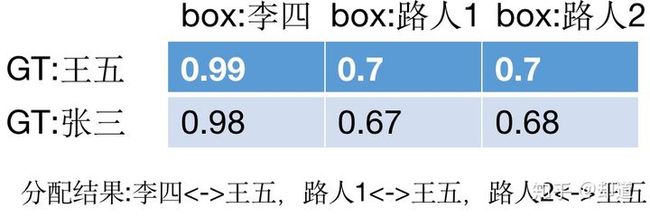
   第3步：box李四负责GT王五，box路人1负责GT王五，box路人2负责GT王五。这一步就导致GT张三被忽略，没有匹配到任何的anchor负责预测，因而需要第四步。
   第4步：对于GT王五，分配到box李四负责，对于GT张三，分配到box李四负责。显然这两步的bbox是有重叠的。即box李四到底是负责哪个GT呢？这和GT的 遍历顺序 有关，谁在后面的顺序遍历的，该box就负责那个GT。
   总之，一个GT可以由多个bbox负责预测，但一个bbox只能负责预测一个GT。

目标检测正负样本区分策略和平衡策略总结（一）

        if self.match_low_quality:
            # Low-quality matching will overwrite the assigned_gt_inds assigned
            # in Step 3. Thus, the assigned gt might not be the best one for
            # prediction.
            # For example, if bbox A has 0.9 and 0.8 iou with GT bbox 1 & 2,
            # bbox 1 will be assigned as the best target for bbox A in step 3.
            # However, if GT bbox 2's gt_argmax_overlaps = A, bbox A's
            # assigned_gt_inds will be overwritten to be bbox B.
            # This might be the reason that it is not used in ROI Heads.
            for i in range(num_gts):
                if gt_max_overlaps[i] >= self.min_pos_iou:
                    if self.gt_max_assign_all:
                        max_iou_inds = overlaps[i, :] == gt_max_overlaps[i]
                        assigned_gt_inds[max_iou_inds] = i + 1
                    else:
                        assigned_gt_inds[gt_argmax_overlaps[i]] = i + 1

【注】加1原因：负样本分配为0，加1是为了不和负样本混淆，后面在为GT分配label时，又进行了索引值减1。

        if gt_labels is not None:
            assigned_labels = assigned_gt_inds.new_full((num_bboxes, ), -1) # 为bbox分配label
            pos_inds = torch.nonzero(
                assigned_gt_inds > 0, as_tuple=False).squeeze()     # [163206]
            if pos_inds.numel() > 0:    # 57
                assigned_labels[pos_inds] = gt_labels[
                    assigned_gt_inds[pos_inds] - 1]
        else:
            assigned_labels = None

        return AssignResult(
            num_gts, assigned_gt_inds, max_overlaps, labels=assigned_labels)

最终，assigned_gt_inds中，忽略样本为-1，负样本为0，正样本为对应的GT索引值+1。（比如有5个GT，某个anchor对应第三个，索引为2，那么分配给该anchor的inds值为3），这样一来，所有正样本分配的值都是大于0的，只要判断大于0即为正样本，用于分配label。
【小结】：

• 如果 anchor 和所有 gt bbox 的最大 iou 值小于 neg_iou_thr，那么该 anchor 就是背景样本；
• 如果 anchor 和所有 gt bbox 的最大 iou 值大于等于 pos_iou_thr，那么该 anchor 就是高质量正样本；
• 如果 gt bbox 和所有 anchor 的最大 iou 值大于等于min_pos_iou，(即使比pos_iou_trh小，但只要大于min_pos_iou，也视为正样本)那么该 gt bbox 所对应的 anchor 也是正样本。每个 gt bbox 都一定有至少一个 anchor 匹配，而一个anchor只能负责预测一个gt；
• 其余样本全部为忽略样本即 anchor 和所有 gt bbox 的最大 iou 值处于 [neg_iou_thr, pos_iou_thr) 区间的 anchor 为忽略样本，不计算 loss

至此，anchor的生成和正负样本匹配策略就分析完成了。

3. BBox Encoder/Decoder

为了更好地平衡多任务分支的loss，在训练过程中引入anchor信息，需要进一步对 bbox 进行编解码操作。RetinaNet使用的是DeltaXYWHBBoxCoder，配置也在bbox_head中，配置文件如下：

        bbox_coder=dict(
            type='DeltaXYWHBBoxCoder',
            target_means=[.0, .0, .0, .0],
            target_stds=[1.0, 1.0, 1.0, 1.0]),

详细代码在：mmdet/core/bbox/coder/delta_xywh_bbox_coder.py

1. 计算proposal和gt的中心坐标、宽高
2. 计算delta值：$dx=\frac{x-x_a}{w_a}$, $dy=\frac{y-y_a}{h_a}$, $dw=log\frac{w}{wa}$, $dh=log\frac{h}{h_a}$。其中，xy、wh表示GT的中心坐标与宽高，xa、ya、wa、ha表示anchor的中心坐标和宽高。

def bbox2delta(proposals, gt, means=(0., 0., 0., 0.), stds=(1., 1., 1., 1.)):
    """Compute deltas of proposals w.r.t. gt.

    We usually compute the deltas of x, y, w, h of proposals w.r.t ground
    truth bboxes to get regression target.
    This is the inverse function of :func:`delta2bbox`.

    Args:
        proposals (Tensor): Boxes to be transformed, shape (N, ..., 4)
        gt (Tensor): Gt bboxes to be used as base, shape (N, ..., 4)
        means (Sequence[float]): Denormalizing means for delta coordinates
        stds (Sequence[float]): Denormalizing standard deviation for delta
            coordinates

    Returns:
        Tensor: deltas with shape (N, 4), where columns represent dx, dy,
            dw, dh.
    """
    assert proposals.size() == gt.size()

    proposals = proposals.float()
    gt = gt.float()
    px = (proposals[..., 0] + proposals[..., 2]) * 0.5
    py = (proposals[..., 1] + proposals[..., 3]) * 0.5
    pw = proposals[..., 2] - proposals[..., 0]
    ph = proposals[..., 3] - proposals[..., 1]

    gx = (gt[..., 0] + gt[..., 2]) * 0.5
    gy = (gt[..., 1] + gt[..., 3]) * 0.5
    gw = gt[..., 2] - gt[..., 0]
    gh = gt[..., 3] - gt[..., 1]

    dx = (gx - px) / pw
    dy = (gy - py) / ph
    dw = torch.log(gw / pw)
    dh = torch.log(gh / ph)
    deltas = torch.stack([dx, dy, dw, dh], dim=-1)

    means = deltas.new_tensor(means).unsqueeze(0)
    stds = deltas.new_tensor(stds).unsqueeze(0)
    deltas = deltas.sub_(means).div_(stds)

    return deltas

4. loss计算

RetinaNet提出Focal loss，用于解决难易样本数量不平衡问题。
Focal loss是Cross Entropy loss 的动态加权版本。交叉熵损失函数如下：

对于正样本，y=1，预测的概率p越大，loss越小；
对于负样本，y=0，预测的概率p越小，loss越小。
但是上述表达式对于正负样本、难易样本都”一视同仁“。（最终总的loss是将每一个样本对应的loss相加，所有样本权重一致）.
(1) 引入参数$\alpha$解决 正负样本不平衡：

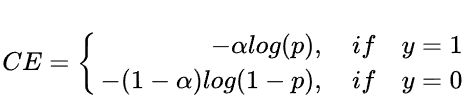
取$\alpha$为0.25。虽然解决了正负样本不平衡问题，但对于难易样本的权重并没有做区分。
（2） 引入参数$\gamma$解决 难易样本：

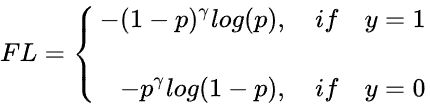
将简单样本（对正样本而言，即预测概率p高）的loss进一步降低，困难样本（对正样本而言，即预测概率p低）的loss进一步升高。

最终的Focal loss形式结合了(1)(2)，如下所示：

$\alpha$是正负样本加权参数，值越大，正样本权重越高；
$\gamma$是难易样本的加权参数，值越大，对错分样本（困难样本权重大）的梯度越大，focal效应越强。
实验表明：$\gamma$取2，$\alpha$取0.25效果最佳。

5分钟理解Focal Loss与GHM——解决样本不平衡利器

Focal loss的配置如下：

        loss_cls=dict(
            type='FocalLoss',
            use_sigmoid=True,
            gamma=2.0,
            alpha=0.25,
            loss_weight=1.0),

Focal loss计算的详细代码：

    pred_sigmoid = pred.sigmoid()
    target = target.type_as(pred)
    pt = (1 - pred_sigmoid) * target + pred_sigmoid * (1 - target)
    focal_weight = (alpha * target + (1 - alpha) *
                    (1 - target)) * pt.pow(gamma)
    loss = F.binary_cross_entropy_with_logits(
        pred, target, reduction='none') * focal_weight
    if weight is not None:
        if weight.shape != loss.shape:
            if weight.size(0) == loss.size(0):
                # For most cases, weight is of shape (num_priors, ),
                #  which means it does not have the second axis num_class
                weight = weight.view(-1, 1)
            else:
                # Sometimes, weight per anchor per class is also needed. e.g.
                #  in FSAF. But it may be flattened of shape
                #  (num_priors x num_class, ), while loss is still of shape
                #  (num_priors, num_class).
                assert weight.numel() == loss.numel()
                weight = weight.view(loss.size(0), -1)
        assert weight.ndim == loss.ndim
    loss = weight_reduce_loss(loss, weight, reduction, avg_factor)
    return loss

而对于回归采用的是 L1 loss：

        loss_bbox=dict(type='L1Loss', loss_weight=1.0)

5. 测试流程

    test_cfg=dict(
        nms_pre=1000,	# 对于每个feature map，nms前按照score大小，保留前1000个box
        min_bbox_size=0,
        score_thr=0.05,	# 分值阈值
        nms=dict(type='nms', iou_threshold=0.5),	# nms阈值
        max_per_img=100)	# 所有feature map的bbox统一进行nms，最后每张图片最多保留100个bbox

总结

本文以RetinaNet为例，结合mmdetection中的代码详细分析了 one-stage detector 的构建以及训练测试流程，尤其是anchor-based方法的anchor生成、正负样本分配、以及bbox编解码策略。此外，还对 Focal loss进行了解析。对于bbox采样策略将在后续的Faster RCNN解读中进行详细分析。

【持续补充更新…】

Reference

[github]openmmlab/mmdetection
轻松掌握 MMDetection 中常用算法(一)：RetinaNet 及配置详解
目标检测正负样本区分策略和平衡策略总结（一）
5分钟理解Focal Loss与GHM——解决样本不平衡利器
Focal Loss for Dense Object Detection