【语义分割】DANet Dual Attention Network for Scene Segmentation

DANet（Dual Attention Network for Scene Segmentation）在语义分割领域多个数据集上取得了STOA的结果，值得大家关注。
【废话两段】
由于之前没跑过语义分割的网络，github上的介绍对于我来说过于简单，花了两天时间才跑通DANET的代码，这里记录一下踩过的坑。
大神可以直接看官方github的内容 https://github.com/junfu1115/DANet
话不多说，我的电脑配置4x2080Ti，操作系统Ubuntu 16.04， 按照模型作者推荐的使用conda搭建的一个python3.6虚拟环境，运行setup.py中的程序包。然后就开始遇到各种问题了

代码调试

RuntimeError: Ninja is required to load C++ extension

google上搜到一个可行的解决方案如下

wget https://github.com/ninja-build/ninja/releases/download/v1.8.2/ninja-linux.zip
sudo unzip ninja-linux.zip -d /usr/local/bin/
sudo update-alternatives --install /usr/bin/ninja ninja /usr/local/bin/ninja 1 --force 

参考：https://github.com/zhanghang1989/PyTorch-Encoding/issues/167

ImportError: No module named ‘ipdb’

这个问题的解决比较直接

pip install ipdb

参考
https://stackoverflow.com/questions/34804121/importerror-no-module-named-ipdb

cityscapes数据集的预处理

这里就比较费功夫了，作者在github只说了到cityscapes上下载数据集然后再转换成19类的数据，具体的操作就只字没提了。
这里作者可能默认大家都是搞语义分割的高手，基本操作就直接忽略了。
在这我就重点分享一下这里的操作细节：

数据集下载

去cityscapes官网的Download页面下载：gtFine_trainvaltest.zip (241MB) [md5]和leftImg8bit_trainvaltest.zip (11GB) [md5]两个数据集

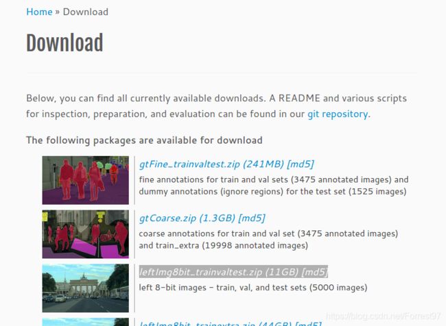
下载完成后解压，关于数据的详细面熟可以在cityscapes数据介绍和处理获得

标签处理

这一步很关键：cityscapes原数据共定义了34类，而DANET只使用了19类。因此需要对监督学习的输出图像进行处理。
cityscapes数据介绍和处理为用户提供了相关的数据处理程序，用户根据自己的需求减少已有的类别，生成新的标签数据集合。真的不是要太贴心！！！
我直接安装cityscapesscripts，然后运行createTrainIdLabelImgs.pyj就可实现新数据的转换

python -m pip install cityscapesscripts
python createTrainIdLabelImgs.py

详细介绍和操作流程可参考：
https://blog.csdn.net/chenzhoujian_/article/details/106874950

生成数据索引txt文件

完成数据转换以后，将数据放到./experiments/cityscapes目录下，距离成功还差最后的数据索引txt文件
根据encoding/datasets/cityscapes.py中可以确定需要生成如下三个重要的文件：
train_fine.txt
val_fine.txt
test.txt
这里直接放我的代码，生成以后就可以按照github上的初始配置训练了

import glob

def make_txtfile(num, mode=None):

    i = 0
    # for the DANET the txt filename
    if mode == "train" or "val":
        txt_name = mode+"_fine"
    else:
        txt_name = mode

    imgs = glob.glob("./datasets/cityscapes/leftImg8bit/"+ mode + "/*/*.png")
    with open("./datasets/cityscapes/"+ txt_name +".txt", "w") as f:
        for path in imgs:
            path = path[22:] # delete "./datasets/cityscapes/"
            data = path + "\t" + path.replace("leftImg8bit", "gtFine").replace("gtFine.png", "gtFine_labelTrainIds.png") + "\n"
            f.write(data)
            i +=1
            if i == num:
                break
    print('write the ', "./datasets/cityscapes/"+ mode+".txt")


if __name__ == '__main__':

    train_num = 2975
    val_num =500
    test_num =1525

    make_txtfile(train_num, mode='train')
    make_txtfile(val_num, mode='val')
    make_txtfile(test_num, mode='test')

参考：
https://blog.csdn.net/chenzhoujian_/article/details/106873451
https://www.cnblogs.com/leviatan/p/10683325.html
https://blog.csdn.net/wang27623056/article/details/106631196

代码解析

个人觉得模型的亮点就是具有两组self-attention机制的注意力模块，所以先介绍两个模块的计算流程，再介绍总体框架的部署情况。

Position Attention Module

数学原理

数学计算流程如下：

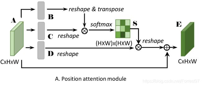
1. 对于深度卷积网络的某一特征层$A\in {\mathbb{R}}^{C\times H\times W}$分别进行卷积操作得到三组新的特征层$\{\mathbf{B},\mathbf{C},\mathbf{D}\}\in {\mathbb{R}}^{C\times H\times W}$
2. 将$\{\mathbf{B},\mathbf{C},\mathbf{D}\}$reshape成 $\{\mathbf{B},\mathbf{C}\}\in {\mathbb{R}}^{C\times N}$，其中$N=H\times W$
3. 将${\mathbf{B}}^{\mathrm{T}}\in {\mathbb{R}}^{N\times C}$与$C\in {\mathbb{R}}^{C\times N}$相乘后得到矩阵$S\in {\mathbb{N}}^{N\times N}$
4. 将$D\in {\mathbb{R}}^{C\times N}$ 与${\mathbf{S}}^{\mathrm{T}}\in {\mathbb{N}}^{N\times N}$相乘后在乘以一个可自学习的的系数$\alpha$
5. 最后残差连接$A\in {\mathbb{R}}^{C\times H\times W}$得到最终的输出特征层$E\in {\mathbb{R}}^{C\times H\times W}$，可表示为$E_j=\alpha {\sum }_{i=1}^N\left(s_{ji}{D}_i\right)+A_j$

我们对关键的$S\in {\mathbb{N}}^{N\times N}$进行注解：
为表示相关系数，即缩放到0-1区间，需要进行一部softmax操作$s_{ji}=\frac{\exp \left(B_i\cdot C_j\right)}{{\sum }_{i=1}^N\exp \left(B_i\cdot C_j\right)}$。此矩阵是用于表示特征层中的第$i$与第$j$特征像素点的相关性，，即计算第$i$与第$j$特征像素点位置处所有通道的内积。这里需要补充一些知识，首先这个操作最先是由何凯明大神在18年CVPR中提出的non-local neural networks。
针对点乘或者内积补充两点：
从线性代数的角度，两向量的内积公式$a\bullet b=|a||b|\cos \theta$与两向量的余弦角相关。而余弦角表示了向量方向的线性相关程度
从统计的角度，两个自变量的内积与协方差相关
$r(X,Y)=\frac{\mathrm{Cov}(X,Y)}{\sqrt{\mathrm{Var}[X]\mathrm{Var}[Y]}}$。协方差表征了两个概率分布的相关性。
说明内积操作的标量能表征相关性，因此对应上面的操作，将第$i$与第$j$特征像素点的所有通道特征数值做内积操作的结果能够表示两个位置相关性。

代码分析

看懂上面的操作下面的代码就很简单了

class PAM_Module(Module):
    """ Position attention module"""
    #Ref from SAGAN
    def __init__(self, in_dim):
        super(PAM_Module, self).__init__()
        self.chanel_in = in_dim
		# 分别得到B,C,D，这里对B和C的输出通道数进行了压缩8倍
        self.query_conv = Conv2d(in_channels=in_dim, out_channels=in_dim//8, kernel_size=1)
        self.key_conv = Conv2d(in_channels=in_dim, out_channels=in_dim//8, kernel_size=1)
        self.value_conv = Conv2d(in_channels=in_dim, out_channels=in_dim, kernel_size=1)
        # gamma 对应上述的alpha
        self.gamma = Parameter(torch.zeros(1))

        self.softmax = Softmax(dim=-1)
    def forward(self, x):
        """
            inputs :
                x : input feature maps( B X C X H X W)
            returns :
                out : attention value + input feature
                attention: B X (HxW) X (HxW)
        """
        m_batchsize, C, height, width = x.size()
        # 矩阵B
        proj_query = self.query_conv(x).view(m_batchsize, -1, width*height).permute(0, 2, 1)
        # 矩阵C
        proj_key = self.key_conv(x).view(m_batchsize, -1, width*height)
        # torch.bmm点积操作
        energy = torch.bmm(proj_query, proj_key)
        # 映射到0-1区间的系数
        attention = self.softmax(energy)
        proj_value = self.value_conv(x).view(m_batchsize, -1, width*height)
        out = torch.bmm(proj_value, attention.permute(0, 2, 1))
        # 矩阵D
        out = out.view(m_batchsize, C, height, width)

        out = self.gamma*out + x
        return out

Channel Attention Module

有了position attention module的理解，接下来的channel attention module就简单很多了。
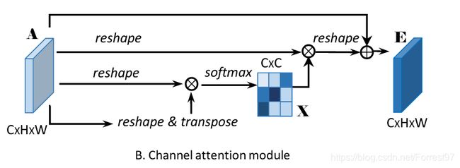这里对着上图，直接看下面的代码。可见，在计算上CAM更为简单和直接，没有中间的卷积操作得到中间特征层，而是由输入特征直接reshape和转置变化以后相乘得到一个$C\times C$的通道权重矩阵。与输入特征A相乘，并乘以系数alpha后进行残差连接得到输出特征E

class CAM_Module(Module):
    """ Channel attention module"""
    def __init__(self, in_dim):
        super(CAM_Module, self).__init__()
        self.chanel_in = in_dim


        self.gamma = Parameter(torch.zeros(1))
        self.softmax  = Softmax(dim=-1)
    def forward(self,x):
        """
            inputs :
                x : input feature maps( B X C X H X W)
            returns :
                out : attention value + input feature
                attention: B X C X C
        """
        m_batchsize, C, height, width = x.size()
        proj_query = x.view(m_batchsize, C, -1)
        proj_key = x.view(m_batchsize, C, -1).permute(0, 2, 1)
        energy = torch.bmm(proj_query, proj_key)
        # 最大值减去原有相关系数矩阵，为什么有这个操作？
        energy_new = torch.max(energy, -1, keepdim=True)[0].expand_as(energy)-energy
        # 大多数的系数都会变得很小
        attention = self.softmax(energy_new)
        proj_value = x.view(m_batchsize, C, -1)
        out = torch.bmm(attention, proj_value)
        out = out.view(m_batchsize, C, height, width)

        out = self.gamma*out + x
        return out

总体网络框架

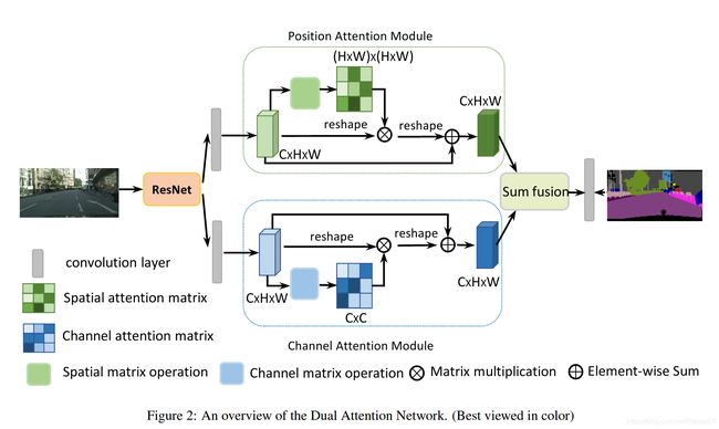
这么看大概能知道框架，由ResNet提取特征后连接一组CAM和PAM模块，但似乎不能了解到细节，随意还是直接上代码：

danat.py

在DANet类中可以看出，确实是由resnet提取特征后，输出layer4的特征，输入到DANetHead中。
注意这里的resnet后两层结构（layer3和4使用了）使用了dilated操作，不会改变特征层的尺寸大小。原文中提到最后一层的特征层尺寸是输入的1/8。保证了特征层保留了更多的细小特征信息。然后在Decoder操作，使用三组upsampling得到与原尺寸相同的语义图。

 class DANet(BaseNet):
    """Fully Convolutional Networks for Semantic Segmentation
    Parameters
    ----------
    nclass : int
        Number of categories for the training dataset.
    backbone : string
        Pre-trained dilated backbone network type (default:'resnet50'; 'resnet50',
        'resnet101' or 'resnet152').
    norm_layer : object
        Normalization layer used in backbone network (default: :class:`mxnet.gluon.nn.BatchNorm`;


    Reference:

        Long, Jonathan, Evan Shelhamer, and Trevor Darrell. "Fully convolutional networks
        for semantic segmentation." *CVPR*, 2015

    """
    def __init__(self, nclass, backbone, aux=False, se_loss=False, norm_layer=nn.BatchNorm2d, **kwargs):
        super(DANet, self).__init__(nclass, backbone, aux, se_loss, norm_layer=norm_layer, **kwargs)
        self.head = DANetHead(2048, nclass, norm_layer)

    def forward(self, x):
        imsize = x.size()[2:]
        _, _, c3, c4 = self.base_forward(x)

        x = self.head(c4)
        x = list(x)
        x[0] = upsample(x[0], imsize, **self._up_kwargs)
        x[1] = upsample(x[1], imsize, **self._up_kwargs)
        x[2] = upsample(x[2], imsize, **self._up_kwargs)

        outputs = [x[0]]
        outputs.append(x[1])
        outputs.append(x[2])
        return tuple(outputs)

这部分程序是对应图中的关键部分。可见除了PAM和CAM模块外，模块前后都都有卷积模块，以及输出以后增加dropout的操作。
还有最后的output是堆叠了sa_output，sc_output以及两者相加求卷积的特征层sasc_output。

• 这里参照原文中的sum_fusion表述，应该只有sasc_output的输出。但是这里同时还输出了sa_output，sc_output。但是源代码运行时无法直接print输出维度

同时注意sasc_output是由sc_conv和sc_conv相加得到的结果

class DANetHead(nn.Module):
    def __init__(self, in_channels, out_channels, norm_layer):
        super(DANetHead, self).__init__()
        inter_channels = in_channels // 4
        self.conv5a = nn.Sequential(nn.Conv2d(in_channels, inter_channels, 3, padding=1, bias=False),
                                   norm_layer(inter_channels),
                                   nn.ReLU())
        
        self.conv5c = nn.Sequential(nn.Conv2d(in_channels, inter_channels, 3, padding=1, bias=False),
                                   norm_layer(inter_channels),
                                   nn.ReLU())

        self.sa = PAM_Module(inter_channels)
        self.sc = CAM_Module(inter_channels)
        self.conv51 = nn.Sequential(nn.Conv2d(inter_channels, inter_channels, 3, padding=1, bias=False),
                                   norm_layer(inter_channels),
                                   nn.ReLU())
        self.conv52 = nn.Sequential(nn.Conv2d(inter_channels, inter_channels, 3, padding=1, bias=False),
                                   norm_layer(inter_channels),
                                   nn.ReLU())

        self.conv6 = nn.Sequential(nn.Dropout2d(0.1, False), nn.Conv2d(inter_channels, out_channels, 1))
        self.conv7 = nn.Sequential(nn.Dropout2d(0.1, False), nn.Conv2d(inter_channels, out_channels, 1))
        self.conv8 = nn.Sequential(nn.Dropout2d(0.1, False), nn.Conv2d(inter_channels, out_channels, 1))

    def forward(self, x):
        feat1 = self.conv5a(x)
        sa_feat = self.sa(feat1)
        sa_conv = self.conv51(sa_feat)
        sa_output = self.conv6(sa_conv)

        feat2 = self.conv5c(x)
        sc_feat = self.sc(feat2)
        sc_conv = self.conv52(sc_feat)
        sc_output = self.conv7(sc_conv)

        feat_sum = sa_conv+sc_conv
        
        sasc_output = self.conv8(feat_sum)

        output = [sasc_output]
        output.append(sa_output)
        output.append(sc_output)
        return tuple(output)