AGS测序下游分析一条龙

1. 表达矩阵

ensembl_matrix.Rdata,原始矩阵

rm(list=ls())
options(stringsAsFactors = F)
library(stringr)  

  a1=read.table('/mnt/AGS_RNA-seq/featureCounts/all.counts.txt',header = T)
  dim(a1)
  a1[1:4,1:4]
  mat= a1[,7:ncol(a1)] 
  rownames(mat)=a1$Geneid
  mat[1:4,1:4]
  keep_feature <- rowSums (mat > 1) > 1
  table(keep_feature)
  mat <- mat[keep_feature, ]
  mat[1:4,1:4]
  dim(mat) 
  colnames(mat)
  #删去62，194组内相关性较差的两组
  #mat <- mat[,-2]
  #mat <- mat[,-5]
  colnames(mat)=c("61","62","63","191","193","194")
  colnames(mat)
  ensembl_matrix=mat
  colnames(ensembl_matrix)
  
  #添加分组信息
  b=read.csv('~/AGS_RNAseq/AGS_4/logs/samples.txt')
  group_list=b$status
  table(group_list)
  save(ensembl_matrix,group_list,file='ensembl_matrix.Rdata')

#samples.txt
Sample,status
61,high
62,high
63,high
191,low
193,low
194,low

2. 数据check，PCA，热图，相关性分析

rm(list = ls()) 
options(stringsAsFactors = F)
load(file = 'ensembl_matrix.Rdata')

# 每次都要检测数据
exprSet=ensembl_matrix
dat=log2(edgeR::cpm(exprSet)+1)
dat[1:4,1:4] 
colnames(exprSet)
table(group_list)

## PCA
dat=t(dat) 
library("FactoMineR")
library("factoextra")  
dat.pca <- PCA(dat , graph = FALSE)#现在dat最后列是group_list，需要重新赋值给一个dat.pca,这个矩阵是不含有分组信息的
fviz_pca_ind(dat.pca,
             geom.ind = "point", # show points only (nbut not "text")
             col.ind =  group_list, # color by groups
             #palette = c("#00AFBB", "#E7B800"),
             addEllipses = TRUE, # Concentration ellipses
             legend.title = "Groups"
)
ggsave('all_samples_PCA_by_type.png')
 

exprSet=ensembl_matrix
dat=log2(edgeR::cpm(exprSet)+1)
dat[1:4,1:4] 
table(group_list)

#表达数据log后较之前均一，看相关性
View(dat)
colnames(dat)
[1] "61"  "62"  "63"  "191" "193" "194"
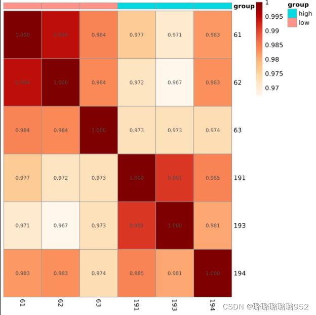
pheatmap::pheatmap(cor(dat))
colD=data.frame(group=group_list)
rownames(colD)=colnames(dat)
pheatmap::pheatmap(cor(dat),annotation_col = colD, 
                   show_rownames = T, 
                   color = colorRampPalette(brewer.pal(9, "OrRd"))(50),
                   cluster_rows = FALSE, 
                   cluster_cols = FALSE, 
                   display_numbers = T, 
                   number_format = "%.3f", ##显示相关系数，三位小数
                   filename = 'cor_log2_all.png')


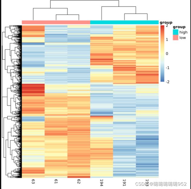
##热图

cg=names(tail(sort(apply(dat,1,sd)),1000))#apply按行（'1'是按行取，'2'是按列取）取每一行的方差，从小到大排序，取最大的1000个
library(pheatmap)
pheatmap(dat[cg,],show_colnames =F,show_rownames = F) #对那些提取出来的1000个基因所在的每一行取出，组合起来为一个新的表达矩阵
n=t(scale(t(dat[cg,]))) # 'scale'可以对log-ratio数值进行归一化
n[n>2]=2 
n[n< -2]= -2
n[1:4,1:4]
pheatmap(n,show_colnames =F,show_rownames = F)
ac=data.frame(group=group_list)
rownames(ac)=colnames(n) 
pheatmap(n,show_colnames =F,show_rownames = F,
         annotation_col=ac)
pheatmap(n,show_colnames =T,show_rownames = F,
         annotation_col=ac,filename = 'heatmap_top1000_sd.png')


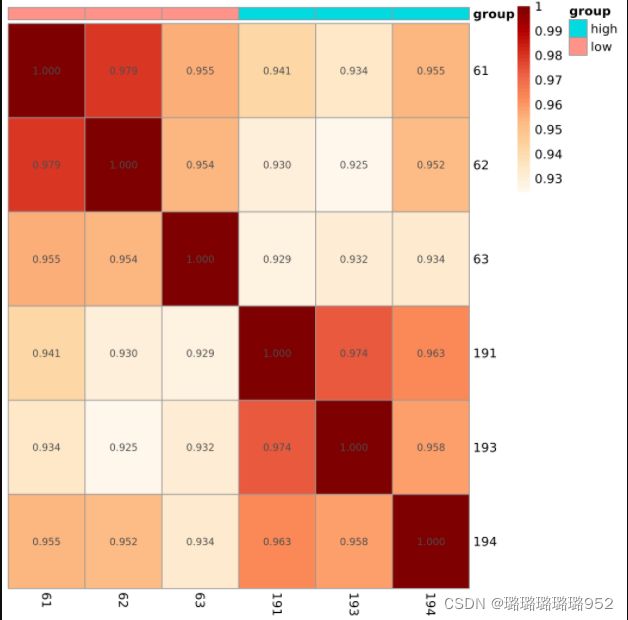
# 相似性，原始矩阵
rm(list = ls())
options(stringsAsFactors = F)
load(file = 'ensembl_matrix.Rdata')

exprSet=ensembl_matrix
colnames(exprSet)
colD=data.frame(group=group_list)
rownames(colD)=colnames(exprSet)
pheatmap::pheatmap(cor(exprSet),annotation_col = colD, 
                   show_rownames = T, 
                   color = colorRampPalette(brewer.pal(9, "OrRd"))(50),
                   cluster_rows = FALSE, 
                   cluster_cols = FALSE, 
                   display_numbers = T, 
                   number_format = "%.3f", 
                   filename = 'cor_all.png')

dim(exprSet)
#[1] 61541     6
exprSet=exprSet[apply(exprSet,1, function(x) sum(x>1) > 3),]
dim(exprSet)
#[1] 18341     6

exprSet=log(edgeR::cpm(exprSet)+1)
dim(exprSet)
exprSet=exprSet[names(sort(apply(exprSet, 1,mad),decreasing = T)[1:500]),]
dim(exprSet)
#[1] 500   6
M=cor(log2(exprSet+1)) 
pheatmap::pheatmap(M,annotation_col = colD)
pheatmap::pheatmap(M,
                   annotation_col = colD,
                   show_rownames = T, 
                   color = colorRampPalette(brewer.pal(9, "OrRd"))(50),
                   cluster_rows = FALSE, 
                   cluster_cols = FALSE, 
                   display_numbers = T, 
                   number_format = "%.3f",  
                   filename = 'cor_top500.png')

log2_all

 top500

3. DESeq2

生成数据：DEG_DEseq2

rm(list = ls())
options(stringsAsFactors = F)
load(file = 'ensembl_matrix.Rdata') 
exprSet=ensembl_matrix 

##可以提前写好完整代码：source('~/AGS_RNAseq/AGS_4/logs/DEG3.R')
##DEG3.R附在最下

table(group_list)  
exprSet[1:4,1:4]
dim(exprSet)
exprSet=exprSet[apply(exprSet,1, function(x) sum(x>1) > 3),]#apply'1'是按行取,'2'是按列取
dim(exprSet) 
 
table(group_list)
##写好的代码中的function：
##run_DEG_RNAseq(exprSet,group_list,
               g1="low",g2="high",
               pro='AGS')

##DESeq2
colnames(exprSet)
library(DESeq2)
g1="low"
g2="high"
colData <- data.frame(row.names=colnames(exprSet), 
                        group_list=group_list) 
dds <- DESeqDataSetFromMatrix(countData = exprSet,
                                colData = colData,
                                design = ~ group_list)
dds <- DESeq(dds)
##会显示标准化进程##
res <- results(dds, 
                 contrast=c("group_list",g2,g1))
mcols(res,use.names= TRUE) # 查看res矩阵每一列的含义
summary(res) # 对res矩阵进行总结
table(res$padj<0.05) # 统计padj小于0.05的数据
resOrdered <- res[order(res$padj),]#按FDR值排序
head(resOrdered)
diff_gene_deseq2 <- subset(res,padj < 0.05 & (log2FoldChange >1 | log2FoldChange < -1)) 
head (diff_gene_deseq2, n=5) # 查看diff_gene_deseq2矩阵的前5行
diff_gene_deseq2 <- row.names(diff_gene_deseq2) # 提取diff_gene_deseq2的行名
head (diff_gene_deseq2, n=5)
resdata <- merge (as.data.frame(res),as.data.frame(counts(dds,normalize=TRUE)),by="row.names",sort=FALSE)
head (resdata,n=5)
write.csv(resdata, file="high_low_diff_gene_deseq2.csv") # 将结果导出

DEG =as.data.frame(resOrdered)
DEG = na.omit(DEG)
nrDEG=DEG
DEG_DEseq2=nrDEG 
nrDEG=DEG_DEseq2[,c(2,6)]
colnames(nrDEG)=c('log2FoldChange','pvalue') 

#离散曲线绘制
png("DESeq2_qc_dispersions.png", 1000, 1000, pointsize=20)
plotDispEsts(dds, main="Dispersion plot")
dev.off()

rld <- rlogTransformation(dds)
exprMatrix_rlog=assay(rld)
    
x=apply(exprMatrix_rlog,1,mean)
y=apply(exprMatrix_rlog,1,mad) 
plot(x,y) 
    
png("DESeq2_RAWvsNORM.png",height = 800,width = 800)
par(cex = 0.7)
n.sample=ncol(exprSet)
if(n.sample>40) par(cex = 0.5)
cols <- rainbow(n.sample*1.2)
par(mfrow=c(2,2))
boxplot(exprSet, col = cols,main="expression value",las=2)
boxplot(exprMatrix_rlog, col = cols,main="expression value",las=2)
hist(as.matrix(exprSet))
hist(exprMatrix_rlog)
dev.off()

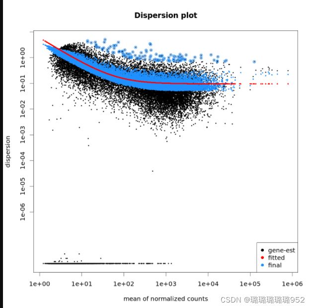
红色离散曲线随着表达水平增加离散值越来越小，说明数据拟合DESeq2模型(11条消息) 哈佛大学——差异表达分析（九）DESeq2步骤描述_零级伪码农的博客-CSDN博客_deseq2差异表达分析

 

4. edgeR

生成data：DEG_edgeR

  library(edgeR)
  g=factor(group_list)
  g=relevel(g,g1)
  d <- DGEList(counts=exprSet,group=g)
  keep <- rowSums(cpm(d)>1) >= 2
  table(keep)
  d <- d[keep, , keep.lib.sizes=FALSE]
  d$samples$lib.size <- colSums(d$counts)
  d <- calcNormFactors(d)
  d$samples
  
  dge=d
  design <- model.matrix(~0+factor(group_list))
  rownames(design)<-colnames(dge)
  colnames(design)<-levels(factor(group_list))
  
  dge <- estimateGLMCommonDisp(dge,design)
  dge <- estimateGLMTrendedDisp(dge, design)
  dge <- estimateGLMTagwiseDisp(dge, design)
  
  fit <- glmFit(dge, design)
  lrt <- glmLRT(fit,  contrast=c(1,-1)) 
  nrDEG=topTags(lrt, n=nrow(dge))
  nrDEG=as.data.frame(nrDEG)
  head(nrDEG)
  DEG_edgeR =nrDEG
  diff_gene_edgeR <- subset(DEG_edgeR,FDR < 0.05 & (logFC >1 | logFC < -1)) 
  head (diff_gene_edgeR, n=5)
  write.csv(diff_gene_edgeR, file="high_low_diff_gene_edgeR.csv") # 将结果导出

  nrDEG=DEG_edgeR[,c(1,5)]
  colnames(nrDEG)=c('log2FoldChange','pvalue')

5.limma

 生成data：DEG_limma_voom

  suppressMessages(library(limma))
  design <- model.matrix(~0+factor(group_list))
  colnames(design)=levels(factor(group_list))
  rownames(design)=colnames(exprSet)
  design
  
  dge <- DGEList(counts=exprSet)
  dge <- calcNormFactors(dge)
  logCPM <- cpm(dge, log=TRUE, prior.count=3)
  
  v <- voom(dge,design,plot=TRUE, normalize="quantile")
  fit <- lmFit(v, design)
  
  group_list
  con=paste0(g2,'-',g1)
  cat(con)
  cont.matrix=makeContrasts(contrasts=c(con),levels = design)
  fit2=contrasts.fit(fit,cont.matrix)
  fit2=eBayes(fit2)
  
  tempOutput = topTable(fit2, coef=con, n=Inf)
  write.csv(tempOutput, file="high_low_limma_DEG_all.csv")
  
  DEG_limma_voom = na.omit(tempOutput)
  head(DEG_limma_voom)
  nrDEG=DEG_limma_voom[,c(1,4)]
  colnames(nrDEG)=c('log2FoldChange','pvalue')

 保存数据：AGS_DEG_results.Rdata

save(DEG_limma_voom,DEG_DEseq2,DEG_edgeR,
       dds,exprSet,group_list,
       file = 'AGS_DEG_results.Rdata')

6.火山图、热图

绘制function

#绘制function
draw_h_v <- function(exprSet,need_DEG,n='DEseq2'){
library(pheatmap)
  exprSet=log(edgeR::cpm(exprSet)+1)
  choose_gene=c(head(rownames(need_DEG),50),
                tail(rownames(need_DEG),50)) ## 50 maybe better
  choose_matrix=exprSet[choose_gene,]
  choose_matrix=t(scale(t(choose_matrix)))
  choose_matrix[choose_matrix>2]=2 
  choose_matrix[choose_matrix< -2]= -2
  choose_matrix[1:4,1:4]
  colD=data.frame(group_list=group_list)
  rownames(colD)=colnames(exprSet)
#热图绘制
  pheatmap(choose_matrix,annotation_col = colD,
           show_rownames = F,
           treeheight_row = 30, #设置聚类线高度
           color = colorRampPalette(c("slategray", "white", "palevioletred2"))(50),
           filename = paste0(n,'_need_DEG_top100_heatmap.png'))
  
#火山图绘制
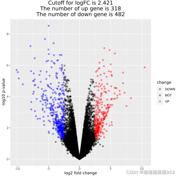
  logFC_cutoff <- with(need_DEG,mean(abs( log2FoldChange)) + 2*sd(abs( log2FoldChange)) )
  # 可以设置logFC_cutoff=1
  
  need_DEG$change = as.factor(ifelse(need_DEG$pvalue < 0.05 & abs(need_DEG$log2FoldChange) > logFC_cutoff,
                                     ifelse(need_DEG$log2FoldChange > logFC_cutoff ,'UP','DOWN'),'NOT')
  )
  this_tile <- paste0('Cutoff for logFC is ',round(logFC_cutoff,3),
                      '\nThe number of up gene is ',nrow(need_DEG[need_DEG$change =='UP',]) ,
                      '\nThe number of down gene is ',nrow(need_DEG[need_DEG$change =='DOWN',])
  )
  library(ggplot2)
  g = ggplot(data=need_DEG, 
             aes(x=log2FoldChange, y=-log10(pvalue), 
                 color=change)) +
    geom_point(alpha=0.4, size=1.75) +
    theme_set(theme_set(theme_bw(base_size=20)))+
    xlab("log2 fold change") + ylab("-log10 p-value") +
    ggtitle( this_tile ) + theme(plot.title = element_text(size=15,hjust = 0.5))+
    scale_colour_manual(values = c('blue','black','red')) ## corresponding to the levels(res$change)
  print(g)
  ggsave(g,filename = paste0(n,'_volcano.png'))
}

#调用绘制function
draw_h_v(exprSet,nrDEG,paste0(pro,'_DEseq2'))
draw_h_v(exprSet,nrDEG,paste0(pro,'_edgeR'))
draw_h_v(exprSet,nrDEG,paste0(pro,'_limma'))

结果如下图，参数可自行修改，如

logFC_cutoff可以设为1

热图参数修改：

(11条消息) pheatmap 参数整理_GeekFocus-CSDN博客_pheatmap 参数详解

常用参数：

scale = "row"归一化

cluster_row = FALSE参数设定不对行进行聚类

legend_breaks参数设定图例显示范围，legend_labels参数添加图例标签

border=FALSE参数去掉边框线

treeheight_row=20和treeheight_col参数设定行和列聚类树的高度，默认为50

cellwidth=15和cellheight参数设定每个热图格子的宽度和高度

main=“主标题”，标题设置

7.KEGG/GO富集

KEGG 

load(file = '~/AGS_RNAseq/AGS_4/all/AGS_DEG_results.Rdata')
load(file = '~/AGS_RNAseq/AGS_4/ensembl_matrix.Rdata')
source('~/AGS_RNAseq/AGS_4/logs/DEG3.R')

#DEG3.R中的function
getDEGs <- function(DEG_DEseq2,DEG_edgeR,DEG_limma_voom,thre_logFC=1,thre_p=0.05){
  head(DEG_DEseq2)
  head(DEG_edgeR)
  head(DEG_limma_voom)
  thre_logFC=1
  thre_p=0.05
  u1=rownames(DEG_DEseq2[with(DEG_DEseq2,log2FoldChange>thre_logFC & padjthre_logFC & FDRthre_logFC & adj.P.Val%
    mutate(pvalue = ifelse(group == "up",-log10(pvalue),log10(pvalue))) %>%
    arrange(group,pvalue)
  double_kegg$Description = factor(double_kegg$Description, 
                                   levels = unique(double_kegg$Description), 
                                   ordered = T)
  head(double_kegg)
  breaks = with(double_kegg, 
                labeling::extended(range(pvalue)[1], range(pvalue)[2],m = 5));breaks
  lm = breaks[c(1,length(breaks))];lm
  KEGG <- ggplot(double_kegg,aes(x=Description,y=pvalue)) +
    geom_segment(aes(x=Description,xend=Description, 
                     y=0,yend=pvalue,color = group),
                 size=5,alpha=0.9) + 
    theme_light() + 
    theme(panel.border = element_rect(fill=NA,color="black", size=0.5, linetype="solid")) + #外框线
    xlab("Pathway") + 
    ylab("-log10(PValue)") + 
    ylim(lm) + 
    scale_y_continuous(breaks = breaks,labels = abs(breaks)) +
    scale_color_brewer(palette = "Pastel2") + # 颜色设置
    labs(title="Pathway Enrichment") + #标题设置
    theme(plot.title = element_text(hjust = 0.5)) + #标题居中
    coord_flip()
  print(KEGG)
  ggsave(KEGG,filename = 'AGS_kegg_up_down.png')

结果：

 

明天继续。