Denoising Diffusion Probabilistic Models简介

概要

Denoising Diffusion Probabilistic Model(DDPM)是一个生成模型，给定一个目标分布，学习模型以便可以从目标分布中采样。
使用马尔科夫链建模。输入是噪声，通过神经网络逐步去噪，最终产生的输出符合目标分布。
生成的数据可以是任意的，可以是图像也可以语音。目前diffusion model主要用于图像生成，所以后面将以图像生成为例介绍。

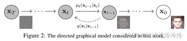
diffusion model分为两个过程：

1. 预定义的前向过程(forward diffusion process)：一步步往图像中加入噪声，直到图像变成纯噪声。该过程的形式和参数都是人为定义的。
2. 需要学习的逆向过程(reverse denoising diffusion process)：一步步从纯噪声中去噪，直到得到图像。该过程用一个可学习的神经网络表示。

前向过程和逆向过程都分为$T$步。图像的生成使用逆向过程。

diffusion model是隐变量模型$p_{\theta }({\mathbf{x}}_0):=\int p_{\theta }({\mathbf{x}}_{0:T})d{\mathbf{x}}_{1:T}$，其中${\mathbf{x}}_0\sim q({\mathbf{x}}_0)$是可观测变量，${\mathbf{x}}_1,{\mathbf{x}}_2,...,{\mathbf{x}}_T$是隐标量并且和可观测变量${\mathbf{x}}_0$有相同的维度。

前向过程

真实数据的分布为$q({\mathbf{x}}_0)$，前向过程是一个预定义的马尔科夫链，其中$q({\mathbf{x}}_t|{\mathbf{x}}_{t-1})$加入高斯噪声：
$$q({\mathbf{x}}_t|{\mathbf{x}}_{t-1})=\mathcal{N}({\mathbf{x}}_t;\sqrt{1-{\beta }_t}{\mathbf{x}}_{t-1},{\beta }_t\mathbf{I})$$其中$0<{\beta }_1<{\beta }_2<...<{\beta }_T<1$是预定义的数值，可以用不同的variance schedule定义。
从$q({\mathbf{x}}_0)$开始，逐步加入高斯噪声，生成${\mathbf{x}}_1,{\mathbf{x}}_2,...,{\mathbf{x}}_T$。如果variance schedule的选择合适，${\mathbf{x}}_T$将是纯高斯噪声。

nice property

根据我们定义的前向过程，一个好的性质是${\mathbf{x}}_t$可以直接采样从${\mathbf{x}}_0$采样得到(高斯的和已经是高斯)，而不需要一步一步地采样:
$$q({\mathbf{x}}_t|{\mathbf{x}}_0)=\mathcal{N}({\mathbf{x}}_t;\sqrt{{\bar{\alpha }}_t}{\mathbf{x}}_0,(1-{\bar{\alpha }}_t)\mathbf{I})$$其中${\alpha }_t:=1-{\beta }_t,{\bar{\alpha }}_t:={\Pi }_{s=1}^t{\alpha }_s$。
因为${\beta }_t$是variance schedule定义的，所以${\alpha }_t$也都是已知的。

逆向过程

逆向过程被定义为一个从$p({\mathbf{x}}_T)=\mathcal{N}({\mathbf{x}}_T;0,\mathbf{I})$出发的马尔科夫链。
前向过程的形式和参数都是预定义的，但后向过程$p({\mathbf{x}}_{t-1}|{\mathbf{x}}_t)$的形式和参数未知的，因为要计算这个条件概率需要知道所有可观测变量的分布。
我们使用一个神经网络来近似这个条件概率，近似概率用$p_{\theta }({\mathbf{x}}_{t-1}|{\mathbf{x}}_t)$表示，其中$\theta$是神经网络的参数，使用梯度下降法优化。
我们并不知道$p({\mathbf{x}}_{t-1}|{\mathbf{x}}_t)$的形式和参数，这里我们假设它是高斯的。高斯分布有两个参数，分别是均值${\mu }_{\theta }$和方差${\Sigma }_{\theta }$，所以逆向过程可以表示为：
$$p_{\theta }({\mathbf{x}}_{t-1}|{\mathbf{x}}_t)=\mathcal{N}({\mathbf{x}}_{t-1};{\mu }_{\theta }({\mathbf{x}}_t,t),{\Sigma }_{\theta }({\mathbf{x}}_t,t))$$使用神经网络学习均值和方差。特别地，DDPM的作者将方差固定为常数，只学习均值。

参数推导

参数推导推导的是逆向过程中的参数。
diffusion model是隐变量模型$p_{\theta }({\mathbf{x}}_0):=\int p_{\theta }({\mathbf{x}}_{0:T})d{\mathbf{x}}_{1:T}$。
考虑最大化log likelihood来学习参数，但因为隐变量模型的likelihood没法直接表示，一般都是采用优化log likelihood的下界variational lower bound (ELBO)。

在diffusion model中，为了方便神经网络优化，我们将最大化问题转换为最小化问题，优化的目标是：
$$\mathbb{E}[-\log p_{\theta }({\mathbf{x}}_0)]\le {\mathbb{E}}_q[-\log \frac{p_{\theta }({\mathbf{x}}_{0:T})}{q({\mathbf{x}}_{1:T}|{\mathbf{x}}_0)}]={\mathbb{E}}_q[-\log p_{(}{\mathbf{x}}_T)-\sum _{t\ge 1}\log \frac{p_{\theta }({\mathbf{x}}_{t-1}|{\mathbf{x}}_t)}{q({\mathbf{x}}_t|{\mathbf{x}}_{t-1})}]:=L$$$L$可以重写为

其中$q({\mathbf{x}}_{t-1}|{\mathbf{x}}_t,{\mathbf{x}}_0)$是高斯分布：

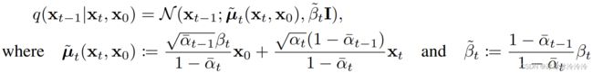
因为$L$中都是高斯函数的KL散度，有闭合(closed form)的表达式。优化时将分别考虑各个$L_t$。

1. 其中因为${\beta }_t$是预定义的，$L_T$是一个常数可以忽略。
2. $L_0$是使用一个单独的离散解码器。
3. $L_{t-1}$可以写为:
   $$L_{t-1}={\mathbb{E}}_{{\mathbf{x}}_0,ϵ}[\frac{1}{2{\sigma }^2}\Vert {\tilde{\mu }}_t({\mathbf{x}}_t,{\mathbf{x}}_0)-{\mu }_{\theta }({\mathbf{x}}_t,t){\Vert }^2]+C$$$L_{t-1}$经过带入公式以及参数化的技巧，优化目标变为
   $${\mathbb{E}}_{{\mathbf{x}}_0,ϵ}[\frac{{\beta }_t^2}{2{\sigma }_t^2{\alpha }_t(1-{\bar{\alpha }}_t)}\Vert ϵ-{ϵ}_{\theta }(\sqrt{{\bar{\alpha }}_t}{\mathbf{x}}_0+\sqrt{(1-{\bar{\alpha }}_t)}ϵ,t){\Vert }^2]$$网络学习的是添加的噪声，${\mu }_{\theta }({\mathbf{x}}_t,t)$可以由下面的公式计算得到$${\mu }_{\theta }({\mathbf{x}}_t,t)=\frac{1}{\sqrt{{\alpha }_t}}({\mathbf{x}}_t-\frac{{\beta }_t}{\sqrt{1-{\bar{\alpha }}_t}}{ϵ}_{\theta }({\mathbf{x}}_{\mathbf{t}},\mathbf{t}))$$

简化

$L_{t-1}$可以进行简化，简化后的目标是：
$${\mathbb{E}}_{{\mathbf{x}}_0,ϵ}\Vert ϵ-{ϵ}_{\theta }(\sqrt{{\bar{\alpha }}_t}{\mathbf{x}}_0,\sqrt{(1-{\bar{\alpha }}_t)}ϵ,t){\Vert }^2$$简化版删去了原有的权重，所以是一个加权的变分界，其减小了$t$较小时的权重。实验显示简化版的优化目标效果更好。

参考资料

NIPS 2020《Denoising Diffusion Probabilistic Models》
Hugging Face blog《The Annotated Diffusion Model》
Lil’Log《What are Diffusion Models?》