opencv学习之：直方图统计、均衡、局部直方图均衡（自适应均衡）

import cv2
import numpy as np
import matplotlib.pyplot as plt
import matplotlib.cm as c
def cv_show(img):
    cv2.imshow("img",img)
    cv2.waitKey(0)
    
    
def cv_read(img_file,gray=True):
    if gray == True:
        return cv2.imread(img_file,0)
    else:
        return cv2.imread(img_file)

• 下文中使用的图像为 lena：
  

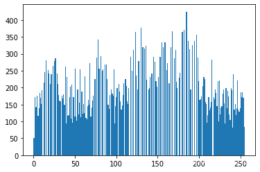
直方图统计

img = cv_read("./img.png")
hist = cv2.calcHist([img],[0],None,[256],[0,256])  ## 计算出的是密度曲线
plt.plot(hist)

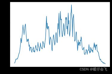
plt.hist(img.ravel(),256)
plt.show()

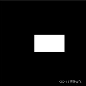
可以通过掩码扣出一部分区域进行直方图统计

# 构造掩码
mask = np.zeros(img.shape,np.uint8)
mask[80:120,80:150] = 255
cv_show(mask)

# 掩码扣到原图上
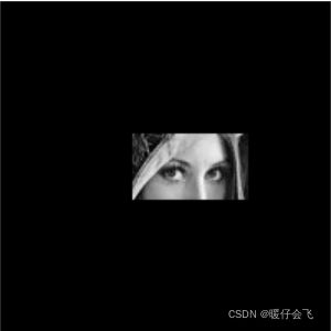
mask_img = np.bitwise_and(img,mask)  # 两种方法都可以求，但略有不同
# mask_img = cv2.bitwise_and(img,img,mask=mask)
cv_show(mask_img)

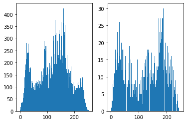
hist_full = cv2.calcHist([img],[0],None,[256],[0,256])
hist_mask = cv2.calcHist([img],[0],mask,[256],[0,256])

fig,(a,b) = plt.subplots(1,2)
a.plot(hist_full)
b.plot(hist_mask)

# 画出分别的统计直方图
fig,(a,b) = plt.subplots(1,2)
a.hist(img.ravel(),256)
b.hist(mask_img[80:120,80:150].ravel(),256)
plt.show()

直方图均衡

• 对于一些没有小细节的图，均衡化之后会显得图更亮，更突出了
• 对于一些有很多小细节的图，均衡化之后会丢失那些原本细节的部分

均衡前

plt.hist(img.ravel(),256)
plt.show()

均衡后

equ = cv2.equalizeHist(img)
plt.hist(equ.ravel(),256)
plt.show()

# 对比结果
show = np.hstack((img,equ))
cv_show(show)

局部均衡化（分小块均衡）：自适应直方图均衡

adaptive = cv2.createCLAHE(clipLimit=2.0, tileGridSize=(8,8))  # 将图分成几乘几

result_adaptive = adaptive.apply(img)
show = np.hstack((img,equ,result_adaptive))
cv_show(show)