【MATLAB学习】北邮电子院MATLAB教程笔记

Matlab 复习

最近在看matplotlib，想到开学用到matlab的机会也很多，于是在Ubuntu20.04上下了个R2021b玩玩，复习matlab对matplotlib也有很大帮助。

课程链接：北京邮电大学MATLAB基础

概述

• MATLAB发展

  由美国Mathworks开发，现在每年发布两个版本a和b，下半年发布的b版更加稳定。
  只有一种数据类型，一种标准的输入输出语句，类似于脚本，不需要编译运行。
  

• MATLAB优点

  除了基本的计算，还提供专业的符号计算，文字处理，可视化建模仿真和实时控制。每个变量都是矩阵，每个元素都是复数。
  自带功能强大的函数，非计算机专业的应该深有体会。
  强大的绘图功能
  强大的工具箱
  

• 工作环境

  进入matlab：
  1.手点快捷方式
  2.Ubuntu进入bin子目录 ./matlab
  退出：
  1.手点
  2.exit，quit
  

  MATLAB窗口：

  命令窗，历史命令窗，当前目录窗，工作空间管理窗，图形窗，文本编辑窗等。

  上图：
  

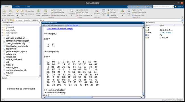
  有关这些窗口个的字体设置可以在preferences中的fonts中自行customize。

• 帮助系统

  help lookfor两个函数。

  help函数弹出帮助文档，lookfor函数查找名称相似的函数。

MATLAB变量

特殊变量

含义	符号
圆周率	pi
机器浮点运算误差限，2.2204e-16	eps
虚数单位	i,j
无穷大	inf
非数	NaN
默认结果存储变量	ans

变量命名规则

所有变量都表示一个矩阵或者一个向量。

1. 变量由大小写英文字幕，数字，下划线组成，但是第一个必须是英文字母。
2. 变量区分大小写
3. 变量不能是MATLAB命令，函数，M文件名，以免引起逻辑运行错误
4. 变量名长度不能超过31

变量的显示

• 格式：MATLAB的数据和计算都以双精度进行，但可以利用format命令调整数据的显示格式
• 变量显示命令：disp函数紧凑格式显示结果。

变量的存取

命令：save load

%格式1：
load 'filename' varname
save 'filename' varname
%格式2：
S = load('filename','format','varname')
save('filename','format','varname')

变量的清除

clear的多种用法：

clear 'varname';
clear var1 var2;
clear all

clear删除内存中的变量，delete删除硬盘上的数据。

检查工作空间中的变量

who %显示前面用过的变量
whos %显示前面用过的变量以及详细特征
%注意：MATLAB中的所有命令和函数都是全小写，否则报错

一维数组的创建与元素提取

1. 直接输入

   直接从键盘输入，分号分隔行与行，逗号或者空格分隔列与列（这样说不太好，逗号或者空格说明数据在同一行比较好）

   >> a = [1;2;3]
   
   a =
   
        1
        2
        3
   
   >> b=[1 2 3]
   
   b =
   
        1     2     3
   
   >> c=[1,2,3]
   
   c =
   
        1     2     3
   

2. 冒号生成法（切片法）

   与py不同的是，python的切片格式是start:stop:step并且stop不能算作最后一个数

   而MATLAB的切片格式为start:step:stop并且stop可以作为最后一个数。

   >> a=1:2:6
   
   a =
   
        1     3     5
   
   >> b=1:6
   
   b =
   
        1     2     3     4     5     6
   

3. 定数线性采样法

   与numpy中的linspace差不多，numpy中的linspace原型是

   def linspace(start, stop, num=50, endpoint=True, retstep=False, dtype=None, axis=0)
   #num指的采样点数，默认50
   #endpoint指最后一个数是否作为采样点，默认真
   >>> a = np.linspace(1, 10, 4)
   >>> a
   array([ 1.,  4.,  7., 10.])
   >>> a = np.linspace(1, 10, 4, endpoint=False)
   >>> a
   array([1.  , 3.25, 5.5 , 7.75])
   

   而MATLAB中的则是：

   linspace(x1,x2,N)
   %将x1，x2（包括两点）线性采样N个点。若不指定N，采样100个点
   >> a = linspace(1,6,6)
   
   a =
   
        1     2     3     4     5     6
   

4. 拼接法

   利用已有的向量拼接创建新的向量。

   %行向量拼接
   a3=[a1,a2]
   %列向量拼接
   b3=[b1;b2]
   %向量抽取
   a4=a3(1:2:end)%这里的end相当于py中的-1索引
   

写个实例：

x1=1:3
x2=linspace(5,20,4)
x=[x1,x2]
y1=[1,3]'
y2=linspace(5,20,4)'
y=[y1;y2]
x3=x(1:2:end)
y3=y(1:2:end)

%%%%%%%%result:
>> T2_2_1

x1 =

     1     2     3


x2 =

     5    10    15    20


x =

     1     2     3     5    10    15    20


y1 =

     1
     3


y2 =

     5
    10
    15
    20


y =

     1
     3
     5
    10
    15
    20


x3 =

     1     3    10    20


y3 =

     1
     5
    15

'是共轭转置运算，之后介绍

小Tips：clc : matlab清屏

二维数组（矩阵）

1. 直接创建

   >> a = [1,2,3;4,5,6;7,8,9]
   
   a =
   
        1     2     3
        4     5     6
        7     8     9
   
   >> a=[1 2 3;4 5 6;7 8 9]
   
   a =
   
        1     2     3
        4     5     6
        7     8     9
   
   >> a=[1,2,3;
   4,5,6;
   7,8,9;]
   
   a =
   
        1     2     3
        4     5     6
        7     8     9
   

2. MATLAB函数创建矩阵

   含义	函数
   全1矩阵	ones()
   全0矩阵	zeros()
   （0，1）区间均匀分布的随机矩阵	rand()
   单位阵	eye()
   均值0，方差1的标准正态分布矩阵	randn()

二维数组元素提取

圆括号，逗号和行，列索引

A=[1 2 3; 4 5 6; 7 8 9]
A(i,j)%提取第i行第j列的元素

A(:,j)：提取第j列为列向量

A(i,:)：提取第i行为行向量

A(:,k:k+m)：提取第k～k+m列为子阵

A(i:i+m,:)：提取第i～i+m行为子阵

A(i:i+m,k:k+m)：提取i～i+m行，k～k+m列为子阵

a=[1,2,3;4,5,6;7,8,9]
a1=a(:,2)
a2=a(2,:)
a3=a(:,1:2)
a4=a(1:2,:)
a5=a(1:2,1:2)
%%%%result：
>> T2_2_2

a =

     1     2     3
     4     5     6
     7     8     9


a1 =

     2
     5
     8


a2 =

     4     5     6


a3 =

     1     2
     4     5
     7     8


a4 =

     1     2     3
     4     5     6


a5 =

     1     2
     4     5

MATLAB字符数组

MATLAB中使用单引号来定义字符数组：

s1='Beijing'
s2='welcome to '

字符数组的拼接：

A='dog'
B='cat'
C=[A,B]
	C='dogcat'

字符数组判空：

isempty(A)
%真1假0，结果类型为logical

矩阵算数运算

1. 矩阵基本算数运算

   • 加法

     $A\pm B$

     注意：要求阶数相同。

     接受矩阵阶数的语句：

     [n,m]=size(A)
     l=length(A)%向量特有
     

   • 乘法

     $A\ast B$

     注意：要求内阶数相同，即A的列数等于B的行数

   • 除法

     矩阵除法比较特殊，就像矩阵乘法是有顺序的，左除右除是不同的两种除法：

     左除：$A\backslash B$

     右除：$B/A$

     原理：
     $$\begin{gathered} A\ast C=B \\ C=A^{-1}\ast B \end{gathered}$$
     当然$A$矩阵是可逆阵，从第一行来看，左右同左乘$A^{-1}$ 可得第二行，就相当于左除$A$矩阵，这就是左除。
     $$\begin{gathered} C\ast A=B \\ C=B\ast A^{-1} \end{gathered}$$
     $A$矩阵可逆，相当于右除$A$矩阵。

   • 幂运算

     A^3

   举个例子：

   A=[1,2; 3,4]
   B=[1,1; 2,2]
   Y1=A+B
   Y2=A-B
   Y3=A*B
   Y4=A\B
   Y5=B/A
   Y6=A^2
   

   结果：

   >> T2_3_1
   
   A =
   
        1     2
        3     4
   
   
   B =
   
        1     1
        2     2
   
   
   Y1 =
   
        2     3
        5     6
   
   
   Y2 =
   
        0     1
        1     2
   
   
   Y3 =
   
        5     5
       11    11
   
   
   Y4 =
   
            0         0
       0.5000    0.5000
   
   
   Y5 =
   
      -0.5000    0.5000
      -1.0000    1.0000
   
   
   Y6 =
   
        7    10
       15    22
   

2. 数组运算

   要求矩阵同阶

   .* %点乘
   ./, .\ %点除
   .^ %点乘方
   

   直接上例子：

   A=[1,2; 3,4]
   B=[1,1; 2,2]
   Y1=A+B
   %Y2=A.+B
   Y3=A.*B
   Y4=A.\B
   Y5=A./B
   Y6=A.^2
   

   结果：

   >> T2_3_2
   
   A =
   
        1     2
        3     4
   
   
   B =
   
        1     1
        2     2
   
   
   Y1 =
   
        2     3
        5     6
   
   
   Y3 =
   
        1     2
        6     8
   
   
   Y4 =
   
       1.0000    0.5000
       0.6667    0.5000
   
   
   Y5 =
   
       1.0000    2.0000
       1.5000    2.0000
   
   
   Y6 =
   
        1     4
        9    16
   

   这里的点左除右除就是简单的对应元素相除。

矩阵的关系运算和逻辑运算

关系运算

运算符：<. <=, >, >=, ==, ~=

真1，假0，类型logical.

当然，只有相同阶数的矩阵才能比较，并生成同阶的logical矩阵。

>> A=magic(3)

A =

     8     1     6
     3     5     7
     4     9     2

>> P=(rem(A,3)==0)

P =

  3×3 logical array

   0   0   1
   1   0   0
   0   1   0

rem函数是用来取余数的

逻辑运算

矩阵的逻辑运算只有三种：

与&或|非~，都是对矩阵的元素进行的运算

>> P=[1,0,1; 0,0,1;1,1,1]

P =

     1     0     1
     0     0     1
     1     1     1

>> U=P|~P

U =

  3×3 logical array

   1   1   1
   1   1   1
   1   1   1

>> all(P)
all(U)
any(P)

ans =

  1×3 logical array

   0   0   1


ans =

  1×3 logical array

   1   1   1


ans =

  1×3 logical array

   1   1   1

其中all，any是针对矩阵的列进行运算的，所以返回的是三个元素的向量。

矩阵元素的处理

矩阵元素取整

function	comment
floor()	向下取整
ceil()	向上取整
round()	四舍五入
fix()	截断小数部分

演示：

>> T2_3_5

A =

    2.3000    2.7000
   -2.3000   -2.7000


A_f =

     2     2
    -3    -3


A_c =

     3     3
    -2    -2


A_r =

     2     3
    -2    -3


A_x =

     2     2
    -2    -2

取模和取余

取模：mod(x,y)

取余：rem(x,y)

说明：当x，y符号相同时，函数结果相同。不同时，rem符号与x相同，mod函数结果与y相同。

a1=mod(8,3)
a2=mod(-8,3)
a3=mod(8,-3)
a4=mod(-8,-3)
a5=rem(8,3)
a6=rem(-8,3)
a7=rem(8,-3)
a8=rem(-8,-3)

结果：

>> T2_3_6

a1 =

     2


a2 =

     1


a3 =

    -1


a4 =

    -2


a5 =

     2


a6 =

    -2


a7 =

     2


a8 =

    -2

行列式，秩，特征值

1. 行列式

   det()

2. 秩

   rank()

3. 迹

   trace()

4. 特征值

   E=eig(A)

   [V,D]=eig(A)

   第一个，E接受A的特征值到一个列向量中。

   第二个，V是A的特征向量，而D是对应的特征值，但是D每个列向量保存一个特征值，所以D是一个对角阵。

演示：

>> T2_4_1

A =

     1    -2     3
     2     3     1
     3    -1    -1


B =

   -45


C =

     3


D =

     3


E =

  -3.1437 + 0.0000i
   3.0719 + 2.2086i
   3.0719 - 2.2086i


V =

  -0.5691 + 0.0000i   0.0023 + 0.5798i   0.0023 - 0.5798i
   0.0517 + 0.0000i   0.7071 + 0.0000i   0.7071 + 0.0000i
   0.8206 + 0.0000i   0.0462 + 0.4021i   0.0462 - 0.4021i


D =

  -3.1437 + 0.0000i   0.0000 + 0.0000i   0.0000 + 0.0000i
   0.0000 + 0.0000i   3.0719 + 2.2086i   0.0000 + 0.0000i
   0.0000 + 0.0000i   0.0000 + 0.0000i   3.0719 - 2.2086i

对非方阵使用这些会导致错误。

矩阵的逆

求逆：

inv()：求满秩方阵的逆

pinv()：求非满秩方阵或者非方阵的伪逆？什么是伪逆，满足：

$$\begin{gathered} ABA=A \\ BAB=B \end{gathered}$$

的矩阵A，称B为A的伪逆。

演示：线性方程组的求解：
$$\begin{array}{r}\{\begin{array}{l}{x}_1-2x_2+3x_3=1\\ 2x_1+3x_2+x_3=2\\ 3x_1-x_2-x_3=4\end{array}\end{array}$$
一般是这么解：$AX=BX=A^{-1}\ast B$

X = inv(A)*B
X = inv(A)*B = A\B

演示：

A=[1,-2,3;2,3,1;3,-1,-1];
B=[1;2;4];
X=inv(A)*B
X1=A\B

结果：

>> T2_4_2

X =

    1.2444
   -0.1111
   -0.1556


X1 =

    1.2444
   -0.1111
   -0.1556

可以左乘逆矩阵和左除效果一样。

矩阵分解与变换

1. 分解

   三角分解（LU分解）：[l,u]=lu(A)

   正交分解（qr分解）：[q,r]=qr(A)

   q：n阶正交方阵

   r：与A同阶上三角阵

   奇异值分解（svd分解）：[u,s,v]=svd(A)

   u：n阶正交阵

   s：n*m阶对角阵，对角元素为A的奇异值

   v：m阶正交方阵

2. 矩阵变换

   共轭转置：‘

   共轭：conj

   转置：conj‘

复矩阵的赋值：

• 依次对元素扶植：

  z=[1+2i,3+4i;5+6i,7+8i]
  

• 分别对实部和虚部赋值：

  z=[1,3;5,7]+[2,4;6,8]*i
  

演示：

z=[1+2i,3+4i;5+6i,7+8i]
z1=z'
z2=conj(z)
z3=conj(z)'

结果：

>> T2_4_3

z =

   1.0000 + 2.0000i   3.0000 + 4.0000i
   5.0000 + 6.0000i   7.0000 + 8.0000i


z1 =

   1.0000 - 2.0000i   5.0000 - 6.0000i
   3.0000 - 4.0000i   7.0000 - 8.0000i


z2 =

   1.0000 - 2.0000i   3.0000 - 4.0000i
   5.0000 - 6.0000i   7.0000 - 8.0000i


z3 =

   1.0000 + 2.0000i   5.0000 + 6.0000i
   3.0000 + 4.0000i   7.0000 + 8.0000i

矩阵的扩展：

a=[1,2,3;4,5,6;7,8,9]
%行扩展：
a(4,3)=6.5
a(5,:)=[5,4,3]
%列扩展
a(:,4)=[5;4;3;2;1]

基本二维曲线绘制

直接来吧：

>> help plot
 plot   Linear plot. 
    plot(X,Y) plots vector Y versus vector X. If X or Y is a matrix,
    then the vector is plotted versus the rows or columns of the matrix,
    whichever line up.  If X is a scalar and Y is a vector, disconnected
    line objects are created and plotted as discrete points vertically at
    X.
 
    plot(Y) plots the columns of Y versus their index.
    If Y is complex, plot(Y) is equivalent to plot(real(Y),imag(Y)).
    In all other uses of plot, the imaginary part is ignored.
 
    Various line types, plot symbols and colors may be obtained with
    plot(X,Y,S) where S is a character string made from one element
    from any or all the following 3 columns:
 
           b     blue          .     point              -     solid
           g     green         o     circle             :     dotted
           r     red           x     x-mark             -.    dashdot 
           c     cyan          +     plus               --    dashed   
           m     magenta       *     star             (none)  no line
           y     yellow        s     square
           k     black         d     diamond
           w     white         v     triangle (down)
                               ^     triangle (up)
                               <     triangle (left)
                               >     triangle (right)
                               p     pentagram
                               h     hexagram
                          
    For example, plot(X,Y,'c+:') plots a cyan dotted line with a plus 
    at each data point; plot(X,Y,'bd') plots blue diamond at each data 
    point but does not draw any line.
 
    plot(X1,Y1,S1,X2,Y2,S2,X3,Y3,S3,...) combines the plots defined by
    the (X,Y,S) triples, where the X's and Y's are vectors or matrices 
    and the S's are strings.  
 
    For example, plot(X,Y,'y-',X,Y,'go') plots the data twice, with a
    solid yellow line interpolating green circles at the data points.
 
    The plot command, if no color is specified, makes automatic use of
    the colors specified by the axes ColorOrder property.  By default,
    plot cycles through the colors in the ColorOrder property.  For
    monochrome systems, plot cycles over the axes LineStyleOrder property.
 
    Note that RGB colors in the ColorOrder property may differ from
    similarly-named colors in the (X,Y,S) triples.  For example, the 
    second axes ColorOrder property is medium green with RGB [0 .5 0],
    while plot(X,Y,'g') plots a green line with RGB [0 1 0].
 
    If you do not specify a marker type, plot uses no marker. 
    If you do not specify a line style, plot uses a solid line.
 
    plot(AX,...) plots into the axes with handle AX.
 
    plot returns a column vector of handles to lineseries objects, one
    handle per plotted line. 
 
    The X,Y pairs, or X,Y,S triples, can be followed by 
    parameter/value pairs to specify additional properties 
    of the lines. For example, plot(X,Y,'LineWidth',2,'Color',[.6 0 0]) 
    will create a plot with a dark red line width of 2 points.
 
    Example
       x = -pi:pi/10:pi;
       y = tan(sin(x)) - sin(tan(x));
       plot(x,y,'--rs','LineWidth',2,...
                       'MarkerEdgeColor','k',...
                       'MarkerFaceColor','g',...
                       'MarkerSize',10)

用汉语解释一下：

plot(X)：

• 如果X是实向量，则纵坐标是向量元素的值，横坐标是向量的索引。注意MATLAB的索引都是从1开始的。
• 如果X是复向量，则相当于plot(real(X),imag(X))，在其他的plot中，虚部都会被忽略。
• 如果X是矩阵，则会绘制多个曲线，将X的列向量当作值（纵坐标），索引当横坐标，有几列就画几个曲线。
• 绘制的曲线是连续的

plot(X,Y)：

• 如果X，Y都是向量，则以X的值作为横坐标，将Y的值作为纵坐标映射到X上，当然，向量长度必须一致。
• 如果X，Y中有矩阵，或者都是矩阵，则将X的列向量作为横坐标，Y的列向量作为纵坐标绘图，并且位置对应，向量元素个数相同。

plot(X,Y,S)：

S是一个字符串，指定曲线的特征，包括颜色，绘制点的形状，绘制线的形状。见前面的说明

plot(X1,Y1,S1,X2,Y2,S2...XN,YN,SN)：

这种情况很简单也很常用，在一张图中绘制很多条曲线。

接下来进行演示：

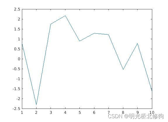
1. plot(y)

   y=5*(rand(1,10)-.5)
   plot(y)
   

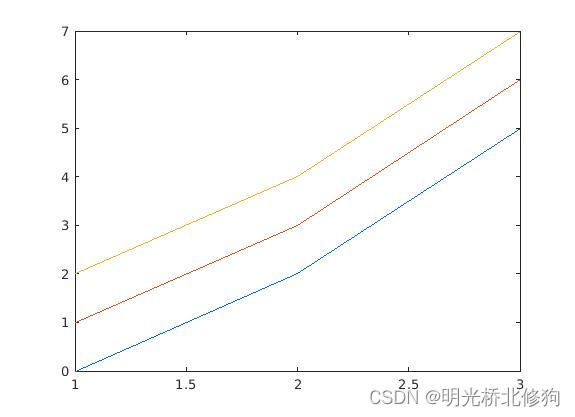
y=[0 1 2;2 3 4;5 6 7]
plot(y)

2. plot(X,Y)

   x=0:0.1:10;
   y=sin(2*x)
   plot(x,y)
   

x=0:0.1:10;
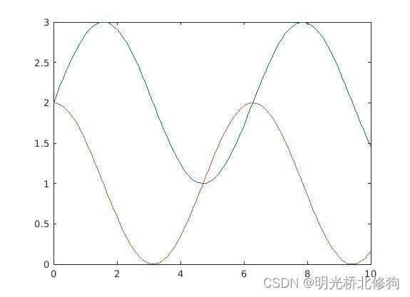
y=[sin(x)+2;cos(x)+1];
plot(x,y)

3. plot(t,[y1;y2;…])

   x=0:0.1:10;
   y1=sin(x)+2;
   y2=cos(x)+1;
   plot(x,[y1;y2]
   

   图和上图相同。

4. plot(t,y1); hold on; plot(t,y2,‘r’)

   x=0:.1:10;
   y1=sin(x)+2;
   y2=cos(x)+1;
   plot(x,y1)
   hold on
   plot(x,y2)
   

   hlod：hold on保持现在的图像，包括坐标范围，曲线的特征等。

   hold off撤销现在绘制的图像，绘制后面的曲线。单个hold切换现在的on或者off。

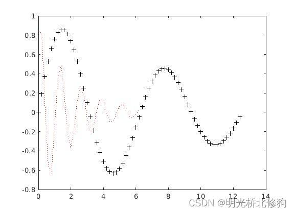
5. plot(x1,y1,s1,x2,y2,s2…)

   t1=0:0.2:4*pi;
   y1=exp(-.1*t1).*sin(t1);
   t2=0:0.2:2*pi;
   y2=exp(-.5*t2).*sin(5*t2+1);
   aplot(t1,y1,'k+',t2,y2,'r:')
   

双纵坐标及多子图的绘制

1. 双纵坐标绘制

   plotyy(x1,y1,x2,y2)

   两条曲线分别以左右两个y轴进行绘制，注意：两个轴的范围可能不同哦。

   上代码：

   x1=0:0.1:5;
   y1=exp(-x1/3);
   x2=0:0.1:5;
   y2=sin(2*x2);
   plotyy(x1,y1,x2,y2)
   title('plotyy exam')
   

这里的title函数指名该图的上标题。

2. 多子图的绘制

   subplot(m,n,p): 绘制m*n张图，p指出第几张图。

   t=0:0.2:4*pi;
   y=exp(-.1*t1).*sin(t1);
   subplot(221),stem(t,y)
   title('stem(t,y)');
   subplot(222),stairs(t,y)
   title('staris(t,y)');
   subplot(223),bar(t,y)
   title('bars(t,y)');
   subplot(2,2,4),fill(t,y,'k')
   title('fill(t,y)');
   

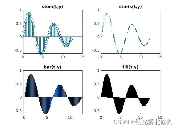
这里的subplot既可以使用逗号将图号隔开，也可以什么都不加。

这里有四个函数绘制不同的曲线，类似于plot：

函数	性质
stem	茎叶图
stairs	梯状图，类似量化图
bar	柱状图
fill	填充图

需要注意的是：fill必须指定S中的颜色。

3. 在多个窗口绘制曲线。

   figure：

   t1=0:0.2:4*pi;
   y1=exp(-.1*t1).*sin(t1);
   y2=exp(-.5*t1).*sin(5*t1+1);
   figure(1)
   plot(t1,y1,'c*')
   figure(2)
   plot(t1,y2,'r:')
   

三维绘制

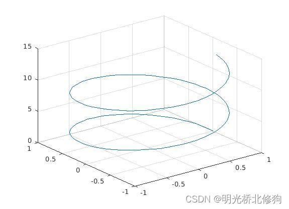
1. 三维曲线绘制

   plot3(x,y,z)

   z=0:0.1:4*pi;
   x=cos(z);
   y=sin(z);
   plot3(x,y,z)
   grid
   

   grid：加上网格状坐标

2. 三维曲面绘制

   mesh：网格状曲面

   surf：给网格填充了颜色的曲面

   x=-8:0.5:8;
   y=x';
   X=ones(size(y))*x;
   Y=y*ones(size(x));
   R=sqrt(X.*X+Y.*Y);
   z=sin(R)./R;
   figure(1),mesh(z)
   figure(2),surf(z)
   

M文件以及函数

在工具栏中可以找到相关的操作，自己看看就好了。

函数的声明举例：

function y=humps(x)
y=1./((x-0.3).^2+0.01)+1./((x-0.9).^2+0.04)-6;

语法：

function [y1,y2...yn]=myfun(x1,x2...xm)

参数为x1，x2…xm，返回y1，y2…yn。

函数代码段可以存在于以下的位置：

1. 只包含函数定义的函数文件中，文件名必须与文件中的第一个函数名一致。
2. 只包含命令和函数定义的脚本文件中。函数必须在文件末尾，脚本文件不能与文件中的函数同名，文件可以包含多个函数定义，函数结束要用end指名。

要使用end结束函数的情况：

• 文件中有函数嵌套
• 函数是函数文件中的局部函数
• 函数是脚本文件中的局部函数

函数参数验证

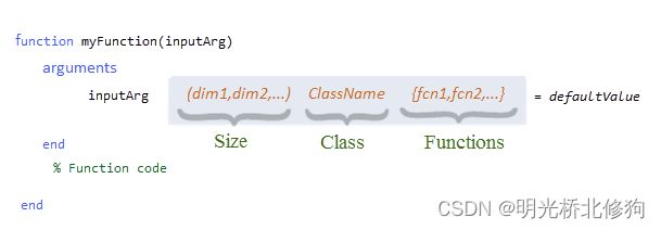
在函数声明后紧跟追加arguments语句段，如图所示。

如果想输入单个元素参数Size段应该为(1,1)，如果想输入向量则应该为(1,:)，这里的接受参数可以是1 * n也可以是n * 1，自动转置。Class指定输入的参数必须是指定类，或者可以转化为指定类

带参数验证的函数，举例：定义一个函数，该函数将输入限制为不包含Inf或者NaN元素的数值向量，使用arguments关键字。

验证函数：

上官网链接自己查看：

验证函数教程

function [m,s] = stat3(x)
	arguments
		x (1,:) {mustBeNumeric, mustBeFinite}
	end
	n = length(x);
	m = avg(x,n);
	s = sqrt(sum((x-m).^2/n));
end

function m = avg(x,n)
	m = sum(x)/n;
end
%(1,:)表示x必须为向量，验证函数{mustBeNumeric, mustBeFinite}将x中元素限制。如果输入Inf或者NaN将报错。

条件控制语句

循环控制语句

发现这两部分没什么可讲的，熟悉C，java，的人没必要看

其他语句

pause

暂停，无参数，等待键盘输入。有参数，暂停多少秒。

input

读入数据，和py一样。

后面的内容我觉得对于matplotlib的学习帮助不大 ，可以掠过了。有需要再看看就好了。