空间分析：5-1.空间分析库PySAL的使用

Pysal与geoda非常相似，一个通过写脚本来实现空间分析，一个通过软件操作来实现空间分析。

Pysal的官网对于自己的介绍是，开源、跨平台的地理空间数据分析库。

http://pysal.org/

 

Pysal能干什么？

空间分析+可视化，就够了。

一、pysal安装

安装非常简单，把相关的包都装一下。

pip install pysal

pip install esda

pip install geopandas

pip install splot

或者打开Pycharm——File——Settings——Python Interpreter。

 

搜索pysal和esda、geopandas、splot，点击install package安装。

 

esda是进行连接分析的，geopandas是对geometry进行矩阵处理的，splot是绘图的。

 

二、官网例子

Pysal官网，最上面就有三个例子：http://pysal.org/

 

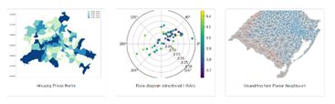
照着这三个例子操作一遍，空间分析就算是入门了。

第一个柏林房价，就是算莫兰指数的。

https://nbviewer.jupyter.org/github/pysal/esda/blob/master/notebooks/Spatial%20Autocorrelation%20for%20Areal%20Unit%20Data.ipynb

第二个是分析局部空间自相关的集聚图，LISA既是Local Indications of Spatial Association。

http://pysal.org/notebooks/explore/giddy/directional.html

第三个是计算空间权重的。

https://nbviewer.jupyter.org/github/pysal/splot/blob/master/notebooks/libpysal_non_planar_joins_viz.ipynb

三、测试数据

可以从git上获取一些数据用来学习：https://github.com/ljwolf/geopython

 

四、demo脚本

我用geopython-master\data里的数据berlin-listings.csv和berlin-neighbourhoods.geojson做了个简单的脚本。

空间权重：

from libpysal.weights.contiguity import Queen
import libpysal
from libpysal import examples
import matplotlib.pyplot as plt
import geopandas as gpd
from splot.libpysal import plot_spatial_weights
gdf = gpd.read_file('data/berlin-neighbourhoods.geojson')
print(gdf.head())
weights = Queen.from_dataframe(gdf)
plot_spatial_weights(weights, gdf)
plt.show()

 

房价分布情况：

import esda

import pandas as pd

import geopandas as gpd

from geopandas import GeoDataFrame

import libpysal as lps

import numpy as np

import matplotlib.pyplot as plt

from shapely.geometry import Point

# %matplotlib inline

gdf = gpd.read_file('data/berlin-neighbourhoods.geojson')

bl_df = pd.read_csv('data/berlin-listings.csv')

geometry = [Point(xy) for xy in zip(bl_df.longitude, bl_df.latitude)]

crs = {'init': 'epsg:4326'}

bl_gdf = GeoDataFrame(bl_df, crs=crs, geometry=geometry)

bl_gdf['price'] = bl_gdf['price'].astype('float32')

sj_gdf = gpd.sjoin(gdf, bl_gdf, how='inner', op='intersects', lsuffix='left', rsuffix='right')

median_price_gb = sj_gdf['price'].groupby([sj_gdf['neighbourhood_group']]).mean()

print(median_price_gb)

gdf = gdf.join(median_price_gb, on='neighbourhood_group')

gdf.rename(columns={'price': 'median_pri'}, inplace=True)

print(gdf.head(15))

pd.isnull(gdf['median_pri']).sum()

gdf['median_pri'].fillna((gdf['median_pri'].mean()), inplace=True)

gdf.plot(column='median_pri')

plt.show()

 

LISA集聚图：

import libpysal
import numpy as np
from giddy.directional import Rose
import matplotlib.pyplot as plt

f = open(libpysal.examples.get_path('spi_download.csv'), 'r')
lines = f.readlines()
f.close()

lines = [line.strip().split(",") for line in lines]
names = [line[2] for line in lines[1:-5]]
data = np.array([list(map(int, line[3:])) for line in lines[1:-5]])

sids = list(range(60))
out = ['"United States 3/"',
      '"Alaska 3/"',
      '"District of Columbia"',
      '"Hawaii 3/"',
      '"New England"','"Mideast"',
       '"Great Lakes"',
       '"Plains"',
       '"Southeast"',
       '"Southwest"',
       '"Rocky Mountain"',
       '"Far West 3/"']
snames = [name for name in names if name not in out]
sids = [names.index(name) for name in snames]
states = data[sids,:]
us = data[0]
years = np.arange(1969, 2009)
rel = states/(us*1.)
gal = libpysal.io.open(libpysal.examples.get_path('states48.gal'))
w = gal.read()
w.transform = 'r'
Y = rel[:, [0, -1]]
# Y.shape
# Y
np.random.seed(100)
r4 = Rose(Y, w, k=4)
r4.plot()
plt.show()

 

五、总结

空间分析，Geoda和pysal，用哪个都行，只要能实现目的，无所谓用软件，还是编写程序。