Chapter 1 - 10: RL in Continuous Spaces
Chapter 1 - 10: RL in Continuous Spaces
1.10.1 Introducing Arpan
1.10.2 Lesson Overview
Reinfoecement learning problems are typically framed as Markov Decision Processor or MDPs. An MDP consists of a set of states S and actions A along with probabilities P, Rewards R and a discount factor gamma. P captures how frequently different transitions and rewards occur, often modeled as a single joint probability where the state and reward at and time step t plus one depend only on the state and action taken at the previous time step t. This characteristic of certain environments is known as the Markov property.
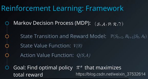
Note that since MDPs are probabilistic in nature, we can’t predict with complete certainty what future rewards we will get and for how long. So, we typically aim for total expected reward. This is where the discount factor gamma comes into play as well. It is used to assign a lower weighted to future rewards when computing state and action values.
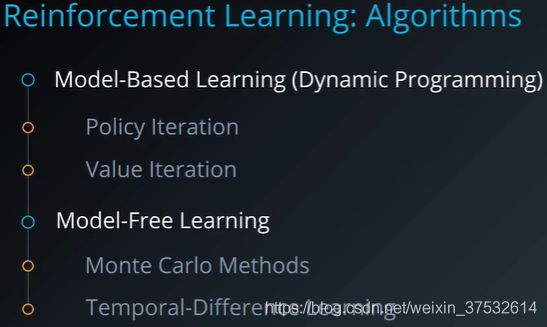
Reinforcement Learning algorithms are generally classified into two grouds. Model-Based approaches such as policy iteration and value iteration require a known transition and reward model. They essentially apply dynamic programming to iteratively compute the desired value functions and optimal policies using that model. On the other hand, model-free approaches including Monte Carlo methods and Temporal-Difference learning don’t require an explicit model. They sample the environment by carrying out exploratory actions and use the experience to directly estimate value functions.
1.10.3 Discrete vs. Continuous Spaces
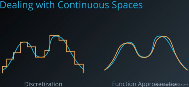
Clearly, we need to modify our representation or algorithms or both to accommodate continuout spaces. The two main strategies we’ll be looking at are Discretization and Function Approximation.
1.10.5 Discretization
1.10.6 Exercise: Discretization
1.10.7 Workspace: Discretization
In this notebook, you will deal with continuous state and action spaces by discretizing them. This will enable you to apply reinforcement learning algorithms that are only designed to work with discrete spaces.
Description
Get an under powered car to the top of a hill (top = 0.5 position)
Observation
Type: Box(2)
| Num | Observation | Min | Max |
|---|---|---|---|
| 0 | position | -1.2 | 0.6 |
| 1 | velocity | -0.07 | 0.07 |
Actions
Type: Discrete(3)
| Num | Action |
|---|---|
| 0 | push left |
| 1 | no push |
| 2 | push right |
Reward
-1 for each time step, until the goal position of 0.5 is reached. As with MountainCarContinuous v0, there is no penalty for climbing the left hill, which upon reached acts as a wall.
Starting State
Random position from -0.6 to -0.4 with no velocity.
Episode Termination
The episode ends when you reach 0.5 position, or if 200 iterations are reached.
1. Import the Necessary Packages
import sys
import gym
import numpy as np

import pandas as pd
import matplotlib.pyplot as plt

# Set plotting options
%matplotlib inline
plt.style.use('ggplot')
np.set_printoptions(precision=3, linewidth=120)

!python -m pip install pyvirtualdisplay
from pyvirtualdisplay import Display
display = Display(visible=0, size=(1400, 900))
display.start()

is_ipython = 'inline' in plt.get_backend()
if is_ipython:
    from IPython import display

plt.ion()
2. An environment that has a continuous state space, but a discrete action space.
A car is on a one-dimensional track, positioned between two “mountains”. The goal is to drive up the mountain on the right; however, the car’s engine is not strong enough to scale the mountain in a single pass. Therefore, the only way to succeed is to drive back and forth to build up momentum.
https://gym.openai.com/videos/2019-10-21–mqt8Qj1mwo/MountainCar-v0/original.mp4
# Create an environment and set random seed
env = gym.make('MountainCar-v0')
env.seed(505);
state = env.reset()
img = plt.imshow(env.render(mode='rgb_array'))
for t in range(1000):
    action = env.action_space.sample()
    # print(action)
    img.set_data(env.render(mode='rgb_array'))
    plt.axis('off')
    display.display(plt.gcf())
    display.clear_output(wait=True)
    state, reward, done, _ = env.step(action)
    print(state, reward, done)
    if done:
        print('Score: ', t+1)
        break

env.close()
# Explore state (observation) space
print("State space:", env.observation_space)
print("- low:", env.observation_space.low)
print("- high:", env.observation_space.high)
# Generate some samples from the state space
print("State space samples:")
print(np.array([env.observation_space.sample() for i in range(10)]))
# Explore the action space
print("Action space:", env.action_space)

# Generate some samples from the action space
print("Action space samples:")
print(np.array([env.action_space.sample() for i in range(10)]))
3. Discretize the State Space with a Uniform Grid (均匀网格)
We will discretize the space using a uniformly-spaced grid. Implement the following function to create such a grid, given the lower bounds (low), upper bounds (high), and number of desired bins along each dimension. It should return the split points for each dimension, which will be 1 less than the number of bins.
For instance, if low = [-1.0, -5.0], high = [1.0, 5.0], and bins = (10, 10), then your function should return the following list of 2 NumPy arrays:
[array([-0.8, -0.6, -0.4, -0.2,  0.0,  0.2,  0.4,  0.6,  0.8]),
 array([-4.0, -3.0, -2.0, -1.0,  0.0,  1.0,  2.0,  3.0,  4.0])]
Note that the ends of low and high are not included in these split points. It is assumed that any value below the lowest split point maps to index 0 and any value above the highest split point maps to index n-1, where n is the number of bins along that dimension.
def create_uniform_grid(low, high, bins=(10, 10)):
    """Define a uniformly-spaced grid that can be used to discretize a space.

    Parameters
    ----------
    low : array_like
        Lower bounds for each dimension of the continuous space.
    high : array_like
        Upper bounds for each dimension of the continuous space.
    bins : tuple
        Number of bins along each corresponding dimension.

    Returns
    -------
    grid : list of array_like
        A list of arrays containing split points for each dimension.
    """
    # TODO: Implement this
    grid = []
    for i, lower_upper in enumerate(zip(low, high)):
        # print(i, lower_upper)
        grid_column = np.linspace(lower_upper[0],[lower_upper[1]], bins[i]+1)[1:-1]
        grid.append(grid_column)

    return grid

low = [-1.0, -5.0]
high = [1.0, 5.0]
create_uniform_grid(low, high)  # [test]
def discretize(sample, grid):
    """Discretize a sample as per given grid.

    Parameters
    ----------
    sample : array_like
        A single sample from the (original) continuous space.
    grid : list of array_like
        A list of arrays containing split points for each dimension.

    Returns
    -------
    discretized_sample : array_like
        A sequence of integers with the same number of dimensions as sample.
    """
    discretized_sample = []
    return list(np.digitize(sample_,grid_) for sample_, grid_ in zip(sample, grid))
    # TODO: Implement this
    '''
        for i, data in enumerate(sample):
        discretized_sample_single = []
        # print(np.digitize(data, grid[i]))
        discretized_sample_single.append(np.digitize(data, grid[i]))
        if i == len(sample) - 0:
            discretized_sample.append(discretized_sample_single)
            print(i)
            print(discretized_sample_single)
    '''


    # return discretized_sample
# Test with a simple grid and some samples
grid = create_uniform_grid([-1.0, -5.0], [1.0, 5.0])
samples = np.array(
    [[-1.0 , -5.0],
     [-0.81, -4.1],
     [-0.8 , -4.0],
     [-0.5 ,  0.0],
     [ 0.2 , -1.9],
     [ 0.8 ,  4.0],
     [ 0.81,  4.1],
     [ 1.0 ,  5.0]])
discretized_samples = np.array([discretize(sample, grid) for sample in samples])
print(discretized_samples[1])
print("\nSamples:", repr(samples), sep="\n")
print("\nDiscretized samples:", repr(discretized_samples), sep="\n")
4. Visualization
It might be helpful to visualize the original and discretized samples to get a sense of how much error you are introducing.
import matplotlib.collections as mc

def visualize_samples(samples, discretized_samples, grid, low=None, high=None):
    """Visualize original and discretized samples on a given 2-dimensional grid."""

    fig, ax = plt.subplots(figsize=(10, 10))

    # Show grid
    ax.xaxis.set_major_locator(plt.FixedLocator(grid[0]))
    ax.yaxis.set_major_locator(plt.FixedLocator(grid[1]))
    ax.grid(True)

    # If bounds (low, high) are specified, use them to set axis limits
    if low is not None and high is not None:
        ax.set_xlim(low[0], high[0])
        ax.set_ylim(low[1], high[1])
    else:
        # Otherwise use first, last grid locations as low, high (for further mapping discretized samples)
        low = [splits[0] for splits in grid]
        high = [splits[-1] for splits in grid]

    # Map each discretized sample (which is really an index) to the center of corresponding grid cell
    grid_extended = np.hstack((np.array([low]).T, grid, np.array([high]).T))  # add low and high ends
    grid_centers = (grid_extended[:, 1:] + grid_extended[:, :-1]) / 2  # compute center of each grid cell
    locs = np.stack(grid_centers[i, discretized_samples[:, i]] for i in range(len(grid))).T  # map discretized samples

    ax.plot(samples[:, 0], samples[:, 1], 'o')  # plot original samples
    ax.plot(locs[:, 0], locs[:, 1], 's')  # plot discretized samples in mapped locations
    ax.add_collection(mc.LineCollection(list(zip(samples, locs)), colors='orange'))  # add a line connecting each original-discretized sample
    ax.legend(['original', 'discretized'])


visualize_samples(samples, discretized_samples, grid, low, high)
Now that we have a way to discretize a state space, let’s apply it to our reinforcement learning environment.
# Create a grid to discretize the state space
state_grid = create_uniform_grid(env.observation_space.low, env.observation_space.high, bins=(10, 10))
state_grid
# Obtain some samples from the space, discretize them, and then visualize them
state_samples = np.array([env.observation_space.sample() for i in range(10)])
discretized_state_samples = np.array([discretize(sample, state_grid) for sample in state_samples])
visualize_samples(state_samples, discretized_state_samples, state_grid,
                  env.observation_space.low, env.observation_space.high)
plt.xlabel('position'); plt.ylabel('velocity');  # axis labels for MountainCar-v0 state space
You might notice that if you have enough bins, the discretization doesn’t introduce too much error into your representation. So we may be able to now apply a reinforcement learning algorithm (like Q-Learning) that operates on discrete spaces. Give it a shot to see how well it works!
5. Q-Learning
Provided below is a simple Q-Learning agent. Implement the preprocess_state() method to convert each continuous state sample to its corresponding discretized representation.
class QLearningAgent:
    """Q-Learning agent that can act on a continuous state space by discretizing it."""

    def __init__(self, env, state_grid, alpha=0.02, gamma=0.99,
                 epsilon=1.0, epsilon_decay_rate=0.9995, min_epsilon=.01, seed=505):
        """Initialize variables, create grid for discretization."""
        # Environment info
        self.env = env
        self.state_grid = state_grid
        self.state_size = tuple(len(splits) + 1 for splits in self.state_grid)  # n-dimensional state space
        self.action_size = self.env.action_space.n  # 1-dimensional discrete action space
        self.seed = np.random.seed(seed)
        print("Environment:", self.env)
        print("State space size:", self.state_size)
        print("Action space size:", self.action_size)

        # Learning parameters
        self.alpha = alpha  # learning rate
        self.gamma = gamma  # discount factor
        self.epsilon = self.initial_epsilon = epsilon  # initial exploration rate
        self.epsilon_decay_rate = epsilon_decay_rate # how quickly should we decrease epsilon
        self.min_epsilon = min_epsilon

        # Create Q-table
        self.q_table = np.zeros(shape=(self.state_size + (self.action_size,)))
        print("Q table size:", self.q_table.shape)

    def preprocess_state(self, state):
        """Map a continuous state to its discretized representation."""
        # TODO: Implement this
        # pass
        return tuple(discretize(state, self.state_grid))

    def reset_episode(self, state):
        """Reset variables for a new episode."""
        # Gradually decrease exploration rate
        self.epsilon *= self.epsilon_decay_rate
        self.epsilon = max(self.epsilon, self.min_epsilon)

        # Decide initial action
        self.last_state = self.preprocess_state(state)
        self.last_action = np.argmax(self.q_table[self.last_state])
        return self.last_action

    def reset_exploration(self, epsilon=None):
        """Reset exploration rate used when training."""
        self.epsilon = epsilon if epsilon is not None else self.initial_epsilon

    def act(self, state, reward=None, done=None, mode='train'):
        """Pick next action and update internal Q table (when mode != 'test')."""
        state = self.preprocess_state(state)
        if mode == 'test':
            # Test mode: Simply produce an action
            action = np.argmax(self.q_table[state])
        else:
            # Train mode (default): Update Q table, pick next action
            # Note: We update the Q table entry for the *last* (state, action) pair with current state, reward
            self.q_table[self.last_state + (self.last_action,)] += self.alpha * \
                (reward + self.gamma * max(self.q_table[state]) - self.q_table[self.last_state + (self.last_action,)])

            # Exploration vs. exploitation
            do_exploration = np.random.uniform(0, 1) < self.epsilon
            if do_exploration:
                # Pick a random action
                action = np.random.randint(0, self.action_size)
            else:
                # Pick the best action from Q table
                action = np.argmax(self.q_table[state])

        # Roll over current state, action for next step
        self.last_state = state
        self.last_action = action
        return action


q_agent = QLearningAgent(env, state_grid)
def run(agent, env, num_episodes=20000, mode='train'):
    """Run agent in given reinforcement learning environment and return scores."""
    scores = []
    max_avg_score = -np.inf
    for i_episode in range(1, num_episodes+1):
        # Initialize episode
        state = env.reset()
        action = agent.reset_episode(state)
        total_reward = 0
        done = False

        # Roll out steps until done
        while not done:
            state, reward, done, info = env.step(action)
            total_reward += reward
            action = agent.act(state, reward, done, mode)

        # Save final score
        scores.append(total_reward)

        # Print episode stats
        if mode == 'train':

            if len(scores) > 100:
                avg_score = np.mean(scores[-100:])
                if avg_score > max_avg_score:
                    max_avg_score = avg_score

            if i_episode % 100 == 0:
                print("\rEpisode {}/{} | Max Average Score: {}".format(i_episode, num_episodes, max_avg_score), end="")
                sys.stdout.flush()

    return scores

scores = run(q_agent, env)
# Plot scores obtained per episode
plt.plot(scores); plt.title("Scores");
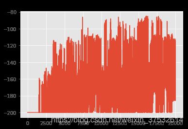
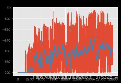
If the scores are noisy, it might be difficult to tell whether your agent is actually learning. To find the underlying trend, you may want to plot a rolling mean of the scores. Let’s write a convenience function to plot both raw scores as well as a rolling mean.
def plot_scores(scores, rolling_window=100):
    """Plot scores and optional rolling mean using specified window."""
    plt.plot(scores); plt.title("Scores");
    rolling_mean = pd.Series(scores).rolling(rolling_window).mean()
    plt.plot(rolling_mean);
    return rolling_mean

rolling_mean = plot_scores(scores)
# Run in test mode and analyze scores obtained
test_scores = run(q_agent, env, num_episodes=100, mode='test')
print("[TEST] Completed {} episodes with avg. score = {}".format(len(test_scores), np.mean(test_scores)))
_ = plot_scores(test_scores, rolling_window=10)
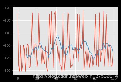
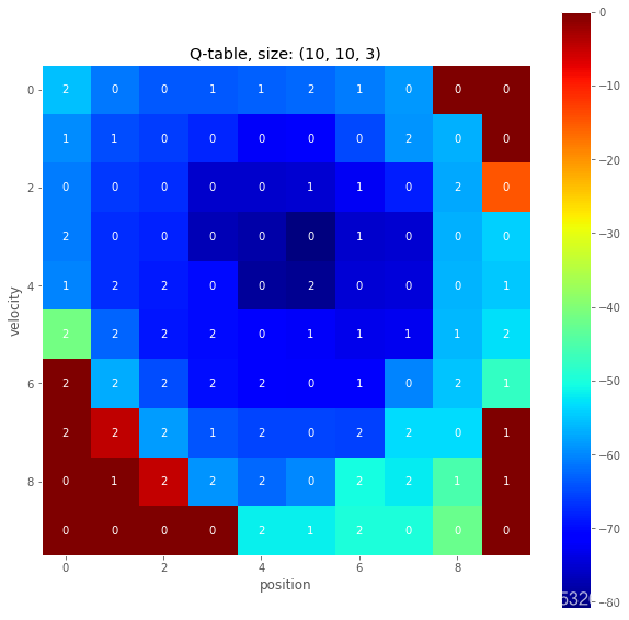
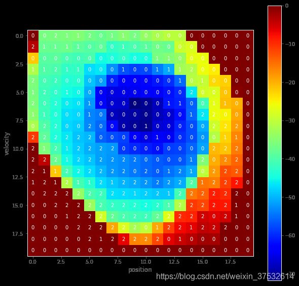
It’s also interesting to look at the final Q-table that is learned by the agent. Note that the Q-table is of size MxNxA, where (M, N) is the size of the state space, and A is the size of the action space. We are interested in the maximum Q-value for each state, and the corresponding (best) action associated with that value.
def plot_q_table(q_table):
    """Visualize max Q-value for each state and corresponding action."""
    q_image = np.max(q_table, axis=2)       # max Q-value for each state
    q_actions = np.argmax(q_table, axis=2)  # best action for each state

    fig, ax = plt.subplots(figsize=(10, 10))
    cax = ax.imshow(q_image, cmap='jet');
    cbar = fig.colorbar(cax)
    for x in range(q_image.shape[0]):
        for y in range(q_image.shape[1]):
            ax.text(x, y, q_actions[x, y], color='white',
                    horizontalalignment='center', verticalalignment='center')
    ax.grid(False)
    ax.set_title("Q-table, size: {}".format(q_table.shape))
    ax.set_xlabel('position')
    ax.set_ylabel('velocity')


plot_q_table(q_agent.q_table)
6. Modify the Grid
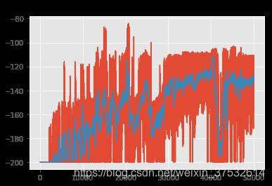
Now it’s your turn to play with the grid definition and see what gives you optimal results. Your agent’s final performance is likely to get better if you use a finer grid, with more bins per dimension, at the cost of higher model complexity (more parameters to learn).
# TODO: Create a new agent with a different state space grid
state_grid_new = create_uniform_grid(env.observation_space.low, env.observation_space.high, bins=(20, 20))
q_agent_new = QLearningAgent(env, state_grid_new)
q_agent_new.scores = []  # initialize a list to store scores for this agent
# Train it over a desired number of episodes and analyze scores
# Note: This cell can be run multiple times, and scores will get accumulated
q_agent_new.scores += run(q_agent_new, env, num_episodes=50000)  # accumulate scores
rolling_mean_new = plot_scores(q_agent_new.scores)
# Run in test mode and analyze scores obtained
test_scores = run(q_agent_new, env, num_episodes=100, mode='test')
print("[TEST] Completed {} episodes with avg. score = {}".format(len(test_scores), np.mean(test_scores)))
_ = plot_scores(test_scores)
# Visualize the learned Q-table
plot_q_table(q_agent_new.q_table)
state = env.reset()
score = 0
for t in range(200):
    action = q_agent_new.act(state, mode='test')
    env.render()
    state, reward, done, _ = env.step(action)
    score += reward
    if done:
        break
print('Final score:', score)
env.close()
1.10.8 Tile Coding
The underlying state space is continuous and two dimensional. We overlay muiltple grids or tilings on top of the space, each slightly offset from each other. Now, any position S in the state space can be coarsely identified by the tiles that it activates. If we assign a bit to each tile, then we can represent out new discretized state as a bit vector, with ones for the tiles that get activated and zeros elsewhere. This, by itself, is a very efficient representation.
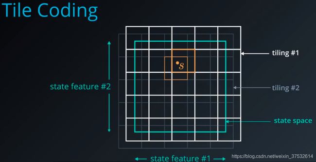
But the genius lies in how the state value function is computed using the scheme. Instead of storing a separate value for each state V of S, it is defined in terms of the bit vector for that state and a weight for each tile.
This ensures nearby locations that share tiles also share some component of state value, effectively smoothing the learned value function.
Tile coding does have some drawbacks. Just like a simple grid based approach we have to manualy select the tile sizes, their offsets, number of tilings.
A more flexible approach is adaptive tile coding, which starts with fairly large tiles, and divides each tile into two whenever appropriate. Basically, we want to split the state space when we realize that we are no longer learning much with the current representation. That is, when our value function isn’t changing. We can stop when we have reached some upper limit on the number of splits or some max iterations.
In order to figure out which tile to split, we have to look at which one is likely to have the greatest effect on the value function. For this, we need to keep track of subtiles and their projected weights. Then, we can pick the tile with the greatest difference between subtile weights.
1.10.10 Workspace: Tile Coding
Tile coding is an innovative way of discretizing a continuous space that enables better generalization compared to a single grid-based approach. The fundamental idea is to create several overlapping grids or tilings; then for any given sample value, you need only check which tiles it lies in. You can then encode the original continuous value by a vector of integer indices or bits that identifies each activated tile.
1. Import the Necessary Packages
# Import common libraries
import sys
import gym
import numpy as np
import matplotlib.pyplot as plt

# Set plotting options
%matplotlib inline
plt.style.use('ggplot')
np.set_printoptions(precision=3, linewidth=120)
2. Specify the Environment, and Explore the State and Action Spaces
We’ll use OpenAI Gym environments to test and develop our algorithms. These simulate a variety of classic as well as contemporary reinforcement learning tasks. Let’s begin with an environment that has a continuous state space, but a discrete action space.
# Create an environment
env = gym.make('Acrobot-v1')
env.seed(505);

# Explore state (observation) space
print("State space:", env.observation_space)
print("- low:", env.observation_space.low)
print("- high:", env.observation_space.high)

# Explore action space
print("Action space:", env.action_space)
Note that the state space is multi-dimensional, with most dimensions ranging from -1 to 1 (positions of the two joints), while the final two dimensions have a larger range. How do we discretize such a space using tiles?
3. Tiling
Let’s first design a way to create a single tiling for a given state space. This is very similar to a uniform grid! The only difference is that you should include an offset for each dimension that shifts the split points.
For instance, if low = [-1.0, -5.0], high = [1.0, 5.0], bins = (10, 10), and offsets = (-0.1, 0.5), then return a list of 2 NumPy arrays (2 dimensions) each containing the following split points (9 split points per dimension):
[array([-0.9, -0.7, -0.5, -0.3, -0.1,  0.1,  0.3,  0.5,  0.7]),
 array([-3.5, -2.5, -1.5, -0.5,  0.5,  1.5,  2.5,  3.5,  4.5])]
Notice how the split points for the first dimension are offset by -0.1, and for the second dimension are offset by +0.5. This might mean that some of our tiles, especially along the perimeter, are partially outside the valid state space, but that is unavoidable and harmless.
def create_tiling_grid(low, high, bins=(10, 10), offsets=(0.0, 0.0)):
    """Define a uniformly-spaced grid that can be used for tile-coding a space.

    Parameters
    ----------
    low : array_like
        Lower bounds for each dimension of the continuous space.
    high : array_like
        Upper bounds for each dimension of the continuous space.
    bins : tuple
        Number of bins or tiles along each corresponding dimension.
    offsets : tuple
        Split points for each dimension should be offset by these values.

    Returns
    -------
    grid : list of array_like
        A list of arrays containing split points for each dimension.
    """
    # TODO: Implement this
    grid = []
    for i, lower_upper in enumerate(zip(low, high)):
        # print(i, lower_upper)
        grid_column = np.linspace(lower_upper[0] ,lower_upper[1] , bins[i]+1)[1:-1] + offsets[i]
        grid.append(grid_column)
    return grid

low = [-1.0, -5.0]
high = [1.0, 5.0]
create_tiling_grid(low, high, bins=(10, 10), offsets=(-0.1, 0.5))  # [test],
You can now use this function to define a set of tilings that are a little offset from each other.
def create_tilings(low, high, tiling_specs):
    """Define multiple tilings using the provided specifications.

    Parameters
    ----------
    low : array_like
        Lower bounds for each dimension of the continuous space.
    high : array_like
        Upper bounds for each dimension of the continuous space.
    tiling_specs : list of tuples
        A sequence of (bins, offsets) to be passed to create_tiling_grid().

    Returns
    -------
    tilings : list
        A list of tilings (grids), each produced by create_tiling_grid().
    """
    # TODO: Implement this

        # print(bins, offset)
    return [create_tiling_grid(low, high, bins, offset) for bins, offset in tiling_specs]


# Tiling specs: [(, ), ...]
tiling_specs = [((10, 10), (-0.066, -0.33)),
                ((10, 10), (0.0, 0.0)),
                ((10, 10), (0.066, 0.33))]
tilings = create_tilings(low, high, tiling_specs)
tilings
It may be hard to gauge whether you are getting desired results or not. So let’s try to visualize these tilings.
from matplotlib.lines import Line2D

def visualize_tilings(tilings):
    """Plot each tiling as a grid."""
    prop_cycle = plt.rcParams['axes.prop_cycle']
    colors = prop_cycle.by_key()['color']
    linestyles = ['-', '--', ':']
    legend_lines = []

    fig, ax = plt.subplots(figsize=(10, 10))
    for i, grid in enumerate(tilings):
        for x in grid[0]:
            l = ax.axvline(x=x, color=colors[i % len(colors)], linestyle=linestyles[i % len(linestyles)], label=i)
        for y in grid[1]:
            l = ax.axhline(y=y, color=colors[i % len(colors)], linestyle=linestyles[i % len(linestyles)])
        legend_lines.append(l)
    ax.grid('off')
    ax.legend(legend_lines, ["Tiling #{}".format(t) for t in range(len(legend_lines))], facecolor='white', framealpha=0.9)
    ax.set_title("Tilings")
    return ax  # return Axis object to draw on later, if needed


visualize_tilings(tilings);
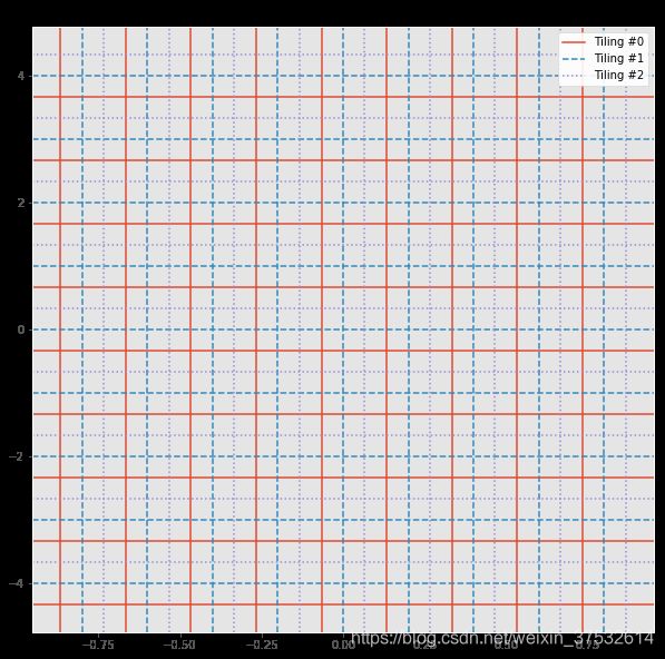
Great! Now that we have a way to generate these tilings, we can next write our encoding function that will convert any given continuous state value to a discrete vector.
4. Tile Encoding
Implement the following to produce a vector that contains the indices for each tile that the input state value belongs to. The shape of the vector can be the same as the arrangment of tiles you have, or it can be ultimately flattened for convenience.
You can use the same discretize() function here from grid-based discretization, and simply call it for each tiling.
def discretize(sample, grid):
    """Discretize a sample as per given grid.

    Parameters
    ----------
    sample : array_like
        A single sample from the (original) continuous space.
    grid : list of array_like
        A list of arrays containing split points for each dimension.

    Returns
    -------
    discretized_sample : array_like
        A sequence of integers with the same number of dimensions as sample.
    """
    # TODO: Implement this
    return tuple(int(np.digitize(sample_,grid_)) for sample_, grid_ in zip(sample, grid))


def tile_encode(sample, tilings, flatten=False):
    """Encode given sample using tile-coding.

    Parameters
    ----------
    sample : array_like
        A single sample from the (original) continuous space.
    tilings : list
        A list of tilings (grids), each produced by create_tiling_grid().
    flatten : bool
        If true, flatten the resulting binary arrays into a single long vector.

    Returns
    -------
    encoded_sample : list or array_like
        A list of binary vectors, one for each tiling, or flattened into one.
    """
    # TODO: Implement this
    return list(discretize(sample, grid) for grid in tilings)


# Test with some sample values
samples = [(-1.2 , -5.1 ),
           (-0.75,  3.25),
           (-0.5 ,  0.0 ),
           ( 0.25, -1.9 ),
           ( 0.15, -1.75),
           ( 0.75,  2.5 ),
           ( 0.7 , -3.7 ),
           ( 1.0 ,  5.0 )]
encoded_samples = [tile_encode(sample, tilings) for sample in samples]
print("\nSamples:", repr(samples), sep="\n")
print("\nEncoded samples:", repr(encoded_samples), sep="\n")
Note that we did not flatten the encoding above, which is why each sample’s representation is a pair of indices for each tiling. This makes it easy to visualize it using the tilings.
from matplotlib.patches import Rectangle

def visualize_encoded_samples(samples, encoded_samples, tilings, low=None, high=None):
    """Visualize samples by activating the respective tiles."""
    samples = np.array(samples)  # for ease of indexing

    # Show tiling grids
    ax = visualize_tilings(tilings)

    # If bounds (low, high) are specified, use them to set axis limits
    if low is not None and high is not None:
        ax.set_xlim(low[0], high[0])
        ax.set_ylim(low[1], high[1])
    else:
        # Pre-render (invisible) samples to automatically set reasonable axis limits, and use them as (low, high)
        ax.plot(samples[:, 0], samples[:, 1], 'o', alpha=0.0)
        low = [ax.get_xlim()[0], ax.get_ylim()[0]]
        high = [ax.get_xlim()[1], ax.get_ylim()[1]]

    # Map each encoded sample (which is really a list of indices) to the corresponding tiles it belongs to
    tilings_extended = [np.hstack((np.array([low]).T, grid, np.array([high]).T)) for grid in tilings]  # add low and high ends
    tile_centers = [(grid_extended[:, 1:] + grid_extended[:, :-1]) / 2 for grid_extended in tilings_extended]  # compute center of each tile
    tile_toplefts = [grid_extended[:, :-1] for grid_extended in tilings_extended]  # compute topleft of each tile
    tile_bottomrights = [grid_extended[:, 1:] for grid_extended in tilings_extended]  # compute bottomright of each tile

    prop_cycle = plt.rcParams['axes.prop_cycle']
    colors = prop_cycle.by_key()['color']
    for sample, encoded_sample in zip(samples, encoded_samples):
        for i, tile in enumerate(encoded_sample):
            # Shade the entire tile with a rectangle
            topleft = tile_toplefts[i][0][tile[0]], tile_toplefts[i][1][tile[1]]
            bottomright = tile_bottomrights[i][0][tile[0]], tile_bottomrights[i][1][tile[1]]
            ax.add_patch(Rectangle(topleft, bottomright[0] - topleft[0], bottomright[1] - topleft[1],
                                   color=colors[i], alpha=0.33))

            # In case sample is outside tile bounds, it may not have been highlighted properly
            if any(sample < topleft) or any(sample > bottomright):
                # So plot a point in the center of the tile and draw a connecting line
                cx, cy = tile_centers[i][0][tile[0]], tile_centers[i][1][tile[1]]
                ax.add_line(Line2D([sample[0], cx], [sample[1], cy], color=colors[i]))
                ax.plot(cx, cy, 's', color=colors[i])

    # Finally, plot original samples
    ax.plot(samples[:, 0], samples[:, 1], 'o', color='r')

    ax.margins(x=0, y=0)  # remove unnecessary margins
    ax.set_title("Tile-encoded samples")
    return ax

visualize_encoded_samples(samples, encoded_samples, tilings);
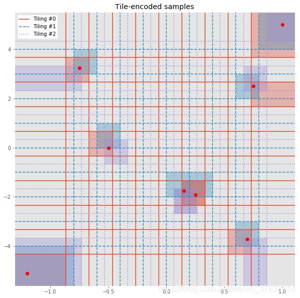
Inspect the results and make sure you understand how the corresponding tiles are being chosen. Note that some samples may have one or more tiles in common.
5. Q-Table with Tile Coding
The next step is to design a special Q-table that is able to utilize this tile coding scheme. It should have the same kind of interface as a regular table, i.e. given a
The
class QTable:
    """Simple Q-table."""

    def __init__(self, state_size, action_size):
        """Initialize Q-table.

        Parameters
        ----------
        state_size : tuple
            Number of discrete values along each dimension of state space.
        action_size : int
            Number of discrete actions in action space.
        """
        self.state_size = state_size
        self.action_size = action_size

        # TODO: Create Q-table, initialize all Q-values to zero
        # Note: If state_size = (9, 9), action_size = 2, q_table.shape should be (9, 9, 2)
        self.q_table = np.zeros(shape=(self.state_size + (self.action_size,)))
        print("QTable(): size =", self.q_table.shape)


class TiledQTable:
    """Composite Q-table with an internal tile coding scheme."""

    def __init__(self, low, high, tiling_specs, action_size):
        """Create tilings and initialize internal Q-table(s).

        Parameters
        ----------
        low : array_like
            Lower bounds for each dimension of state space.
        high : array_like
            Upper bounds for each dimension of state space.
        tiling_specs : list of tuples
            A sequence of (bins, offsets) to be passed to create_tilings() along with low, high.
        action_size : int
            Number of discrete actions in action space.
        """
        self.tilings = create_tilings(low, high, tiling_specs)
        self.state_sizes = [tuple(len(splits)+1 for splits in tiling_grid) for tiling_grid in self.tilings]
        # print(self.state_sizes)
        self.action_size = action_size
        self.q_tables = [QTable(state_size, self.action_size) for state_size in self.state_sizes]
        print("TiledQTable(): no. of internal tables = ", len(self.q_tables))

    def get(self, state, action):
        """Get Q-value for given  pair.

        Parameters
        ----------
        state : array_like
            Vector representing the state in the original continuous space.
        action : int
            Index of desired action.

        Returns
        -------
        value : float
            Q-value of given  pair, averaged from all internal Q-tables.
        """
        # TODO: Encode state to get tile indices
        encoded_state = tile_encode(state, self.tilings)
        # TODO: Retrieve q-value for each tiling, and return their average
        value = 0.0
        for idx, q_table in zip(encoded_state, self.q_tables):
            value += q_table.q_table[tuple(idx + (action,))]
        value /= len(self.q_tables)
        return value
        pass

    def update(self, state, action, value, alpha=0.1):
        """Soft-update Q-value for given  pair to value.

        Instead of overwriting Q(state, action) with value, perform soft-update:
            Q(state, action) = alpha * value + (1.0 - alpha) * Q(state, action)

        Parameters
        ----------
        state : array_like
            Vector representing the state in the original continuous space.
        action : int
            Index of desired action.
        value : float
            Desired Q-value for  pair.
        alpha : float
            Update factor to perform soft-update, in [0.0, 1.0] range.
        """
        # TODO: Encode state to get tile indices
        encoded_state = tile_encode(state, self.tilings)
        # TODO: Update q-value for each tiling by update factor alpha
        for idx, q_table in zip(encoded_state, self.q_tables):
            value_ = q_table.q_table[tuple(idx + (action,))]  # current value
            q_table.q_table[tuple(idx + (action,))] = alpha * value + (1.0 - alpha) * value_


# Test with a sample Q-table
tq = TiledQTable(low, high, tiling_specs, 2)
s1 = 3; s2 = 4; a = 0; q = 1.0
print("[GET]    Q({}, {}) = {}".format(samples[s1], a, tq.get(samples[s1], a)))  # check value at sample = s1, action = a
print("[UPDATE] Q({}, {}) = {}".format(samples[s2], a, q)); tq.update(samples[s2], a, q)  # update value for sample with some common tile(s)
print("[GET]    Q({}, {}) = {}".format(samples[s1], a, tq.get(samples[s1], a)))  # check value again, should be slightly updated
class QLearningAgent:
    """Q-Learning agent that can act on a continuous state space by discretizing it."""

    def __init__(self, env, tq, alpha=0.02, gamma=0.99,
                 epsilon=1.0, epsilon_decay_rate=0.9995, min_epsilon=.01, seed=0):
        """Initialize variables, create grid for discretization."""
        # Environment info
        self.env = env
        self.tq = tq
        self.state_sizes = tq.state_sizes           # list of state sizes for each tiling
        self.action_size = self.env.action_space.n  # 1-dimensional discrete action space
        self.seed = np.random.seed(seed)
        print("Environment:", self.env)
        print("State space sizes:", self.state_sizes)
        print("Action space size:", self.action_size)

        # Learning parameters
        self.alpha = alpha  # learning rate
        self.gamma = gamma  # discount factor
        self.epsilon = self.initial_epsilon = epsilon  # initial exploration rate
        self.epsilon_decay_rate = epsilon_decay_rate   # how quickly should we decrease epsilon
        self.min_epsilon = min_epsilon

    def reset_episode(self, state):
        """Reset variables for a new episode."""
        # Gradually decrease exploration rate
        self.epsilon *= self.epsilon_decay_rate
        self.epsilon = max(self.epsilon, self.min_epsilon)

        self.last_state = state
        Q_s = [self.tq.get(state, action) for action in range(self.action_size)]
        self.last_action = np.argmax(Q_s)
        return self.last_action

    def reset_exploration(self, epsilon=None):
        """Reset exploration rate used when training."""
        self.epsilon = epsilon if epsilon is not None else self.initial_epsilon

    def act(self, state, reward=None, done=None, mode='train'):
        """Pick next action and update internal Q table (when mode != 'test')."""
        Q_s = [self.tq.get(state, action) for action in range(self.action_size)]
        # Pick the best action from Q table
        greedy_action = np.argmax(Q_s)
        if mode == 'test':
            # Test mode: Simply produce an action
            action = greedy_action
        else:
            # Train mode (default): Update Q table, pick next action
            # Note: We update the Q table entry for the *last* (state, action) pair with current state, reward
            value = reward + self.gamma * max(Q_s)
            self.tq.update(self.last_state, self.last_action, value, self.alpha)

            # Exploration vs. exploitation
            do_exploration = np.random.uniform(0, 1) < self.epsilon
            if do_exploration:
                # Pick a random action
                action = np.random.randint(0, self.action_size)
            else:
                # Pick the greedy action
                action = greedy_action

        # Roll over current state, action for next step
        self.last_state = state
        self.last_action = action
        return action
n_bins = 5
bins = tuple([n_bins]*env.observation_space.shape[0])
offset_pos = (env.observation_space.high - env.observation_space.low)/(3*n_bins)

tiling_specs = [(bins, -offset_pos),
                (bins, tuple([0.0]*env.observation_space.shape[0])),
                (bins, offset_pos)]

tq = TiledQTable(env.observation_space.low,
                 env.observation_space.high,
                 tiling_specs,
                 env.action_space.n)
agent = QLearningAgent(env, tq)
def run(agent, env, num_episodes=10000, mode='train'):
    """Run agent in given reinforcement learning environment and return scores."""
    scores = []
    max_avg_score = -np.inf
    for i_episode in range(1, num_episodes+1):
        # Initialize episode
        state = env.reset()
        action = agent.reset_episode(state)
        total_reward = 0
        done = False

        # Roll out steps until done
        while not done:
            state, reward, done, info = env.step(action)
            total_reward += reward
            action = agent.act(state, reward, done, mode)

        # Save final score
        scores.append(total_reward)

        # Print episode stats
        if mode == 'train':
            if len(scores) > 100:
                avg_score = np.mean(scores[-100:])
                if avg_score > max_avg_score:
                    max_avg_score = avg_score
            if i_episode % 100 == 0:
                print("\rEpisode {}/{} | Max Average Score: {}".format(i_episode, num_episodes, max_avg_score), end="")
                sys.stdout.flush()
    return scores

scores = run(agent, env)
def plot_scores(scores, rolling_window=100):
    """Plot scores and optional rolling mean using specified window."""
    plt.plot(scores); plt.title("Scores");
    rolling_mean = pd.Series(scores).rolling(rolling_window).mean()
    plt.plot(rolling_mean);
    return rolling_mean

rolling_mean = plot_scores(scores)
1.10.11 Coarse Coding
Coarse coding is just like tile coding, but uses a sparser set of features to encode the state space. Image dropping a bunch of circles on your 2D continuous state space. Take any state S which is a position in this space, and mark all the circles that it belongs to. Prepare a bit vector(位向量) with a one for those circles and 0 for the rest. And that’s your sparse coding representation of the state.
Using smaller circles results in less generalization across the space. The learning algorithms has to work a bit longer, but you have greater effective resolution.
A nutural extension to this idea is to use the distance from the center of each circle as a measure of how active that feature is.
This measure or response can be made to fall off smoothly using a Gaussian or a bell-shaped curve centered on the circle. which is known as radial basis function.
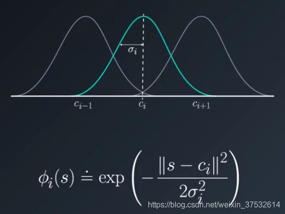
The number of feautres can be drastically reduced this way.
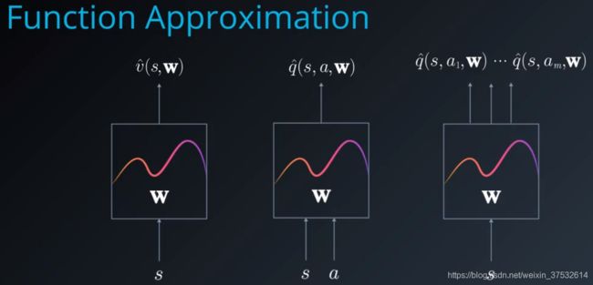
1.10.11 Function Approximation
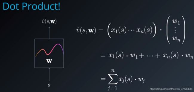
1.10.11 Linear Function Approximation
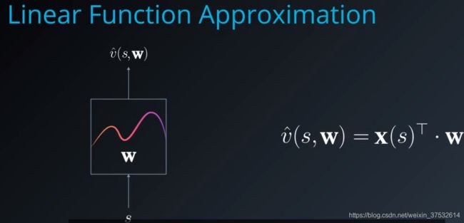
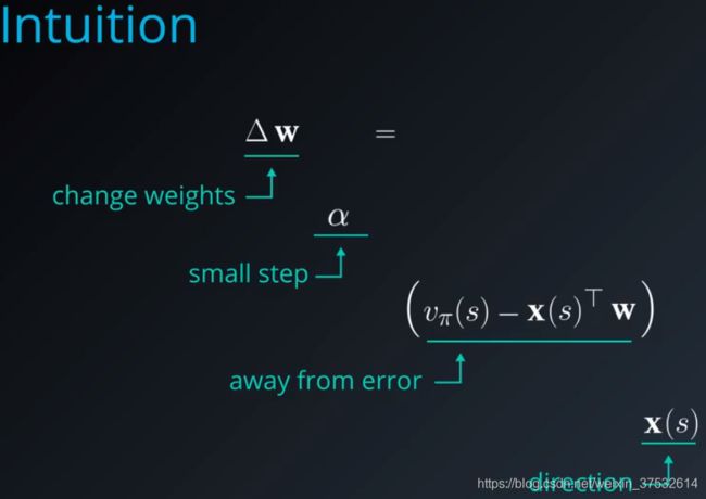
Let’s assume you have initialized these weights randomly and computed the value of a state v hat (s,w). How would you tweak w to bring the approximation closer and closer to the true function? Sounds like a numerical optimization problem. We can use gradient descent to find the optimal parameter vector. We want to reduce or minimize the difference between the true value function v pi and the approximate value function v hat.
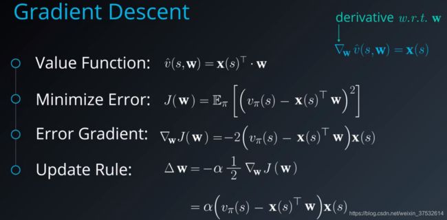
Note that we remove the expection operator here to focus on the error gradient indicated by a single state s, which we assume has been chosen stochastically. If we are able to sample enough states, we can come close to the expected value.
