计算机视觉(五)图像检索与识别
文章目录
-
- 一、原理及流程
-
- 1.1 概述
- 1.2 算法描述
- 1.3 算法流程
- 1.4 TF-IDF
- 二、代码实现
-
- 2.1 代码
- 2.2 运行及结果
一、原理及流程
1.1 概述
如果不寻找新方法,那么:
250,000 张图像 ~ 310亿个图像对
– 每个图相对2秒 匹配 500台并行计算机需要1年才能完成计算
因此使用一种基于Bag-of-words models的Bof,即Bag of features。
图像纹理是什么?纹理是指图像中的重复模式,或纹理基元组成的结构。因此可以将图像的这种结构,生成类似词库的东西,用来提供检索图像
1.2 算法描述
视觉词袋模型( Bag-of-features )是当前计算机视觉领域中较为常用的图像表示方法。
视觉词袋模型来源于词袋模型(Bag-of-words),词袋模型最初被用在文本分类中,将文档表示成特征矢量。它的基本思想是假定 对于一个文本,忽略其词序和语法、句法, 仅仅将其看做是一些词汇的集合, 而文本中的每个词汇都是独立的。简单说就是讲每篇文档都看成一个袋子 (因为里面装的都是词汇,
所以称为词袋,Bag of words即因此而来)然后看这个袋子里装的都是些什么词汇,将其分类。
如果文档中猪、 马、牛、羊、山谷、土地、拖拉机这样的词汇多些,而银行、大厦、汽车、公园这样的词汇少些, 我们就倾向于判断它是一 篇描绘乡村的文档,而不是描述城镇的。
Bag of Feature也是借鉴了这种思路,只不过在图像中,我们抽出的不再是一个个word, 而是 图像的关键特征Feature,所以研究人员将它更名为Bag of Feature.Bag of Feature在检索中的算法流程和分类几乎完全一样,唯一的区别在于,对于原始的BOF特征,也就是直方图向量,我们引入TF_IDF权值。

1.3 算法流程
1,特征提取
提取图像的基本特征

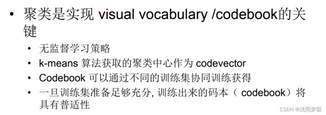
2,学习 “视觉词典(visual vocabulary)

根据这些特征,把有同属性的特征划分为同一类
可以使用K-means 聚类算法
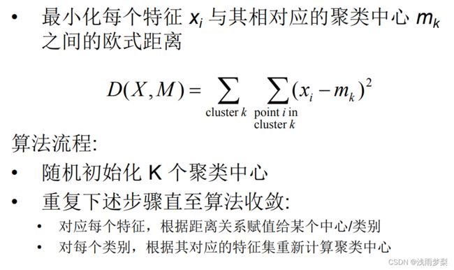

3,针对输入特征集,根据视觉词典进行量化

4,把输入图像转化成视觉单词(visual words)的频率直方图

1.4 TF-IDF
根据特征投票应该赋予相应的权重。这些权重的设置就是TF-IDF
公式如下:
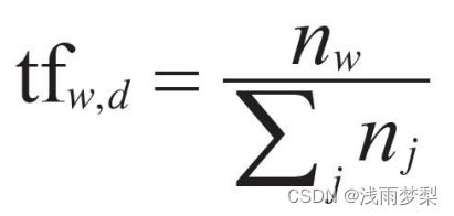

如果一个 关键词只在很少的网页中出现,我们通过它就 容易锁定搜索目标,它的 权重也就应该 大。反之如果一个词在大量网页中出现,我们看到它仍然 不是很清楚要找什么内容,因此它应该 小
二、代码实现
2.1 代码
1、给训练图像集生成词汇字典。生成字典之前要先提取图像的 SIFT特征点
# -*- coding: utf-8 -*-
import pickle
from PCV.imagesearch import vocabulary
from PCV.tools.imtools import get_imlist
from PCV.localdescriptors import sift

#获取图像列表

imlist = get_imlist('E:/CV/img/c6/')
nbr_images = len(imlist)

#获取特征列表
featlist = [imlist[i][:-3]+'sift' for i in range(nbr_images)]

#提取文件夹下图像的sift特征
for i in range(nbr_images):
    sift.process_image(imlist[i], featlist[i])

#生成词汇
voc = vocabulary.Vocabulary('ukbenchtest')
voc.train(featlist, 1000, 10)
#保存词汇
# saving vocabulary
with open('E:/CV/img/c6/vocabulary.pkl', 'wb') as f:
    pickle.dump(voc, f)
print('vocabulary is:', voc.name, voc.nbr_words)
2、将图像添加到数据库
# -*- codeing =utf-8 -*-

import pickle
from PCV.imagesearch import imagesearch
from PCV.localdescriptors import sift
import sqlite3
from PCV.tools.imtools import get_imlist

# 获取图像列表

imlist = get_imlist('E:/CV/img/c6/')
nbr_images = len(imlist)
# 获取特征列表
featlist = [imlist[i][:-3] + 'sift' for i in range(nbr_images)]

# load vocabulary
# 载入词汇

with open('E:/CV/img/c6/vocabulary.pkl', 'rb') as f:
    voc = pickle.load(f)
# 创建索引
indx = imagesearch.Indexer('testImaAdd.db', voc)
indx.create_tables()

# go through all images, project features on vocabulary and insert
# 遍历所有的图像,并将它们的特征投影到词汇上
for i in range(nbr_images)[:17]:
    locs, descr = sift.read_features_from_file(featlist[i])
    indx.add_to_index(imlist[i], descr)
# commit to database
# 提交到数据库
indx.db_commit()

con = sqlite3.connect('testImaAdd.db')
print(con.execute('select count (filename) from imlist').fetchone())
print(con.execute('select * from imlist').fetchone())
3、图像检索测试
import pickle
from PCV.localdescriptors import sift
from PCV.imagesearch import imagesearch
from PCV.geometry import homography
from PCV.tools.imtools import get_imlist
# load image list and vocabulary
# 载入图像列表
imlist = get_imlist('E:/CV/img/c6/') # 存放数据集的路径
nbr_images = len(imlist)
# 载入特征列表
featlist = [imlist[i][:-3] + 'sift' for i in range(nbr_images)]
# 载入词汇
with open('E:/CV/img/c6/vocabulary.pkl', 'rb') as f: # 存放模型的路径
voc = pickle.load(f)
src = imagesearch.Searcher('testImaAdd.db', voc)
# index of query image and number of results to return
# 查询图像索引和查询返回的图像数
q_ind = 3
nbr_results = 5
# regular query
# 常规查询(按欧式距离对结果排序)
res_reg = [w[1] for w in src.query(imlist[q_ind])[:nbr_results]]
print('top matches (regular):', res_reg)
# load image features for query image
# 载入查询图像特征
q_locs, q_descr = sift.read_features_from_file(featlist[q_ind])
fp = homography.make_homog(q_locs[:, :2].T)
# RANSAC model for homography fitting
# 用单应性进行拟合建立RANSAC模型
model = homography.RansacModel()
rank = {}
# load image features for result
# 载入候选图像的特征
for ndx in res_reg[1:]:
locs, descr = sift.read_features_from_file(featlist[ndx]) # because 'ndx' is a rowid of the DB that starts at 1
# get matches
# 获取匹配数 # get matches执行完后会出现两张图片
matches = sift.match(q_descr, descr)
ind = matches.nonzero()[0]
ind2 = matches[ind]
tp = homography.make_homog(locs[:, :2].T)
# compute homography, count inliers. if not enough matches return empty list
# 计算单应性,对内点技术。如果没有足够的匹配书则返回空列表
try:
H, inliers = homography.H_from_ransac(fp[:, ind], tp[:, ind2], model, match_theshold=4)
except:
inliers = []
# store inlier count
rank[ndx] = len(inliers)
# sort dictionary to get the most inliers first
# 将字典排序,以首先获取最内层的内点数
sorted_rank = sorted(rank.items(), key=lambda t: t[1], reverse=True)
res_geom = [res_reg[0]] + [s[0] for s in sorted_rank]
print('top matches (homography):', res_geom)
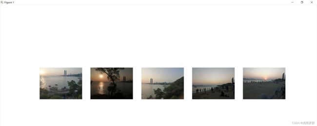
# 显示查询结果
imagesearch.plot_results(src, res_reg[:8]) # 常规查询
imagesearch.plot_results(src, res_geom[:8]) # 重排后的结果
2.2 运行及结果
1、图像及生成的sift特征点如下:

2、查询结果:查询图像在最左边,后面都是按图像列表检索的前5幅图像。