监督学习week 1: 单变量线性回归optional_lab收获记录
目录
1.cost function
2.gradient&gradient descent
①compute_gradient
②Gradient Descent
③使用:
④画图&预测
1.cost function
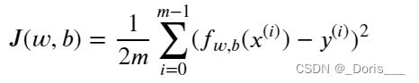
#Function to calculate the cost
def compute_cost(x, y, w, b):

    m = x.shape[0]
    cost = 0

    for i in range(m):
        f_wb = w * x[i] + b
        cost = cost + (f_wb - y[i])**2
    total_cost = 1 / (2 * m) * cost

    return total_cost
2.gradient&gradient descent
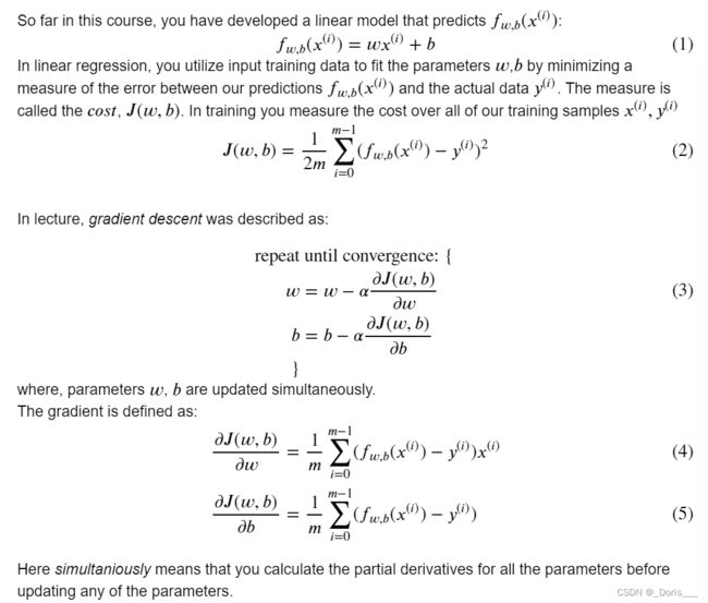
①compute_gradient
def compute_gradient(x, y, w, b):
    m = x.shape[0]
    dj_dw = 0
    dj_db = 0

    for i in range(m):
        f_wb = w * x[i] + b
        dj_dw_i = (f_wb - y[i]) * x[i]
        dj_db_i = f_wb - y[i]
        dj_db += dj_db_i
        dj_dw += dj_dw_i
    dj_dw = dj_dw / m
    dj_db = dj_db / m

    return dj_dw, dj_db
②Gradient Descent
def gradient_descent(x, y, w_in, b_in, alpha, num_iters,
 cost_function, gradient_function):

    w = copy.deepcopy(w_in) # avoid modifying global w_in
    # An array to store cost J and w's at each iteration primarily for graphing later
    J_history = []
    p_history = []
    b = b_in
    w = w_in

    for i in range(num_iters):
        # Calculate the gradient and update the parameters using gradient_function
        dj_dw, dj_db = gradient_function(x, y, w , b)

        # Update Parameters using equation (3) above
        b = b - alpha * dj_db
        w = w - alpha * dj_dw

        # Save cost J at each iteration
        if i<100000:      # prevent resource exhaustion
            J_history.append( cost_function(x, y, w , b))
            p_history.append([w,b])
        # Print cost every at intervals 10 times or as many iterations if < 10
        if i% math.ceil(num_iters/10) == 0:
            print(f"Iteration {i:4}: Cost {J_history[-1]:0.2e} ",
                  f"dj_dw: {dj_dw: 0.3e}, dj_db: {dj_db: 0.3e}  ",
                  f"w: {w: 0.3e}, b:{b: 0.5e}")

    return w, b, J_history, p_history #return w and J,w history for graphing
注意:函数的参数调用其他函数(本质上,也是一个对象->可以当做参数使用)
③使用:
# initialize parameters
w_init = 0
b_init = 0
# some gradient descent settings
iterations = 10000
tmp_alpha = 1.0e-2
# run gradient descent
w_final, b_final, J_hist, p_hist =
gradient_descent(x_train ,y_train, w_init, b_init,
 tmp_alpha, iterations, compute_cost, compute_gradient)
print(f"(w,b) found by gradient descent: ({w_final:8.4f},{b_final:8.4f})")
④画图&预测
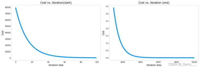
# plot cost versus iteration
fig, (ax1, ax2) = plt.subplots(1, 2, constrained_layout=True, figsize=(12,4))
ax1.plot(J_hist[:100])
ax2.plot(1000 + np.arange(len(J_hist[1000:])), J_hist[1000:])
ax1.set_title("Cost vs. iteration(start)");  ax2.set_title("Cost vs. iteration (end)")
ax1.set_ylabel('Cost')            ;  ax2.set_ylabel('Cost')
ax1.set_xlabel('iteration step')  ;  ax2.set_xlabel('iteration step')
plt.show()