混合模型简介与高斯混合模型
高斯混合模型
混合模型概述
In statistics, a mixture model is a probabilistic model for representing the presence of subpopulations within an overall population, without requiring that an observed data set should identify the sub-population to which an individual observation belongs. Formally a mixture model corresponds to the mixture distribution that represents the probability distribution of observations in the overall population. However, while problems associated with “mixture distributions” relate to deriving the properties of the overall population from those of the sub-populations, “mixture models” are used to make statistical inferences about the properties of the sub-populations given only observations on the pooled population, without sub-population identity information.
从统计学角度来说,一个混合模型就是一种概率模型,用于表示总体当中子总体的存在,而不需要观测数据集识别出这个观测数据属于哪一个子总体(子分布)。
形式上讲,对应混合分布的一个混合模型,就代表了这个总体的概率密度分布。然而,但需要从子总体的性质推导总体的一些性质时,混合模型能够直接根据总体池的观测值来对子总体的特性进行统计推断,而不需要知道他们的归属信息(属于哪一个子总体)。
Mixture Model Structure
A typical finite-dimensional mixture model is a hierarchical model consisting of the following components:
- N random variables that are observed, each distributed according to a mixture of K components, with the components belonging to the same parametric family of distributions (e.g., all normal, all Zipfian, etc.) but with different parameters
- N random latent variables specifying the identity of the mixture component of each observation, each distributed according to a K-dimensional categorical distribution
- A set of K mixture weights, which are probabilities that sum to 1.
- A set of K parameters, each specifying the parameter of the corresponding mixture component. In many cases, each “parameter” is actually a set of parameters. For example, if the mixture components are Gaussian distributions, there will be a mean and variance for each component. If the mixture components are categorical distributions (e.g., when each observation is a token from a finite alphabet of size V), there will be a vector of V probabilities summing to 1.
In addition, in a Bayesian setting, the mixture weights and parameters will themselves be random variables, and prior distributions will be placed over the variables. In such a case, the weights are typically viewed as a K-dimensional random vector drawn from a Dirichlet distribution (the conjugate prior of the categorical distribution), and the parameters will be distributed according to their respective conjugate priors.
一个典型的有限维度的混合模型是一个分层的模型,有着如下的components:
- N N N个被观测的随机变量random variables,每个随机变量都按 K K K个子分布(
component)构成的混合模型而分布,这些子分布都属于同一类分布,但是具体的参数值不同。 - N N N个隐变量
latent variables,每一个隐变量都说明了对应的随机变量所属的子分布是哪一个。每一个隐变量都按 K K K维分类分布(即隐变量的取值只有 K K K个) - K K K个混合权重,每个混合权重指定了某个子分布所占的总体的权重。混合权重的和加起来应等于1.
- K K K个参数组,每一个参数组都对应着一个子分布。如高斯混合模型中,每个参数组中的参数有均值和方差。
此外,在贝叶斯假设下,混合权重和参数组将本身就是随机变量,每个都会有一个先验分布。在这种情况下,混合权重可以被视为一个 K K K维的随机向量,由狄利克雷分布(分类分布的共轭先验)得出,而参数组将根据各自的先验共轭分布而分布。(关于先验概率与后验概率在这里不表。)
从数学角度出发,一个基础的参数化的混合模型可以被以下参数所描述:
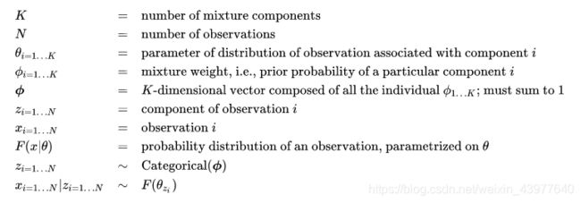
参数解读:
K K K 表示mixture component的个数,即混合分布中子分布的个数。
N N N 表示被观测的随机变量的个数。
θ i = 1... K {\theta _{{\rm{i}} = 1...K}} θi=1...K表示第 i i i个子分布component的参数值。
ϕ i = 1... K {\phi _{{\rm{i}} = 1...K}} ϕi=1...K表示混合权重,即某个具体的子分布component的先验概率。
Φ \Phi Φ表示由 ϕ i = 1... K {\phi _{{\rm{i}} = 1...K}} ϕi=1...K组成的K维向量,和为1.
z i = 1... N {z _{{\rm{i}} = 1...N}} zi=1...N表示第 i i i个观测值所属的component(子分布)。
x i = 1... N {x _{{\rm{i}} = 1...N}} xi=1...N表示第 i i i个观测的随机变量。
F ( x ∣ θ ) F(x|\theta ) F(x∣θ)表示某个被观测的随机变量在参数组为 θ \theta θ下的概率分布。
z i = 1... N {z _{{\rm{i}} = 1...N}} zi=1...N服从以 Φ \Phi Φ为概率的分类分布(共 K K K类)。 即: z i = 1... N ∼ C a t e g o r i c a l ( Φ ) {z_{i = 1...N}} \sim Categorical(\Phi ) zi=1...N∼Categorical(Φ)
x i = 1... N ∣ z i = 1... N {x_{i = 1...N}}|{z_{i = 1...N}} xi=1...N∣zi=1...N 服从 F ( θ z i ) F(\theta _{z_i} ) F(θzi),即随机变量 x i x_i xi服从其对应component(子分布) z i z_i zi的参数组 θ z i \theta _{z_i} θzi指定的概率分布。
注意:以上参数都是在不是在贝叶斯假设下的。
在贝叶斯假设下,所有参数都与随机变量相关,如下图:
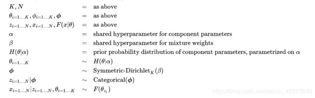
参数解读:
K K K: 同上
N N N: 同上
θ i = 1... K \theta _{i=1...K} θi=1...K: 同上
ϕ i = 1... K \phi _{i=1...K} ϕi=1...K: 同上
Φ \Phi Φ: 同上
z i = 1... N z _{i=1...N} zi=1...N:同上
x i = 1... N x_{i=1...N} xi=1...N:同上
F ( x ∣ θ ) F(x|\theta) F(x∣θ):同上
α \alpha α:各子分布component参数的共用的超参数
β \beta β: 混合权重的共用的超参数
H ( θ ∣ α ) H(\theta|\alpha) H(θ∣α): 子分布component参数的先验概率分布,基于参数 α \alpha α。
θ i = 1... K \theta _{i=1...K} θi=1...K: 服从概率分布 H ( θ ∣ α ) H(\theta|\alpha) H(θ∣α),即 θ i = 1... K ∼ H ( θ ∣ α ) \theta _ {i=1...K} \sim H(\theta|\alpha) θi=1...K∼H(θ∣α)
Φ \Phi Φ: 服从 S y m m e t r i c − D i r i c h l e t K ( β ) Symmetric-Dirichlet _K(\beta) Symmetric−DirichletK(β)分布。
z i = 1... N ∣ Φ z_{i=1...N}|\Phi zi=1...N∣Φ:服从 C a t e g o r i c a l ( ϕ ) Categorical(\phi) Categorical(ϕ),即以 Φ \Phi Φ为概率的分类分布。
x i = 1... N ∣ z i = 1... N , θ i = 1... K x_{i=1...N}|z_{i=1...N},\theta_{i=1...K} xi=1...N∣zi=1...N,θi=1...K:服从 F ( θ z i ) F(\theta_{z_i}) F(θzi)的分布。
我们使用 F F F和 H H H来对观测值和参数进行任意描述。一般来说, H H H是 F F F的共轭先验。两个最常见的 F F F的选择是:高斯分布,即正态分布(对实值观测值),或者是分类分布(对离散观测值)。其他常见的可以作为混合组件的概率分布有:
- 二项分布
Binomial distribution: 对于某一事物总数固定,统计其positive occurrence。如投票等。 - 多项分布
Multinomial distribution: 类似于二项分布,不过事情的结果可能不止有两个。 - 负二项分布
Negative binomial distribution: 对于二项分布类型的观测值,感兴趣的是在某个给定的次数的positive结果出现前,negative结果出现的次数。 - 泊松分布
Poisson distribution:统计某一事件在给定时间内发生的次数,该事件具有固定的发生率。 - 指数分布
Exponential distribution:某个事件下一次出现所需要的的时间的分布,该事件具有固定的发生率。 - 对数正态分布
Log-normal distribution: 用于那些假定呈指数增长的正实数,如收入或者价格。 - 多元正态分布
Multivariate normal distribution:即多元高斯分布。结果向量的每一个分量都是一个高斯分布。 - 多元t分布
Multivariate Student's-t distribution:用于重尾相关结果的向量。 - 伯努利分布值的向量,对应于例如黑白图像,每个值代表一个像素,可应用于手写识别。
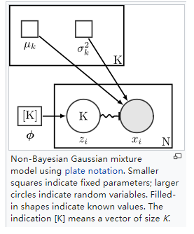
非贝叶斯假设下的高斯混合模型
其各个参数为:

对应上文很容易理解,不再赘述。
图示:
贝叶斯假设下的高斯混合模型
其各个参数为:
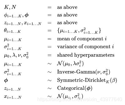
其中值得特殊说明的是:
μ 0 , λ , ν , σ 0 2 {\mu _0},\lambda ,\nu ,\sigma _0^2 μ0,λ,ν,σ02: 是 θ \theta θ即 μ \mu μ与 σ \sigma σ共享的超参数。
μ i = 1... K \mu_{i=1...K} μi=1...K: μ i = 1... K ∼ N ( μ 0 , λ σ i 2 ) \mu_{i=1...K} \sim N(\mu_0,\lambda\sigma _i^2) μi=1...K∼N(μ0,λσi2),即参数 μ \mu μ服从以 m u 0 , λ σ i 2 mu_0,\lambda\sigma _i^2 mu0,λσi2为参数的高斯分布。
σ i = 1... K 2 \sigma_{i=1...K}^2 σi=1...K2: σ i = 1... K 2 ∼ I n v e r s e − G a m m a ( ν , σ 0 2 ) \sigma_{i=1...K}^2 \sim Inverse-Gamma(\nu,\sigma_0^2) σi=1...K2∼Inverse−Gamma(ν,σ02)。
多元高斯混合模型
一个贝叶斯高斯混合模型常常被推广去拟合未知的参数向量(下面用粗体表示),或者多元正态分布。在多元分布中(即对具有 N N N个随机变量的向量 x \bm{x} x),我们可以使用高斯混合模型的先验分布的矢量估计来对该 x \bm{x} x进行建模:
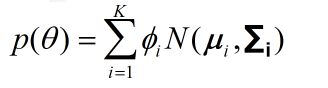
其中第 i i i个向量子分布component被权重为 ϕ i {\phi _i} ϕi,方差为 μ \bm{\mu} μ,协方差矩阵为 ∑ i \bm{\sum _i} ∑i的正态分布所定义。为了将这个先验分布纳入贝叶斯估计,这个先验要与已知的分布 p ( x ∣ θ ) p(\bm{x}|\bm{\theta}) p(x∣θ)相乘,该分布是数据 x \bm{x} x在待估参数 θ \bm{\theta} θ上的分布。根据如上阐述,那么后验分布 p ( θ ∣ x ) p(\bm{\theta}|\bm{x}) p(θ∣x)也是一个高斯混合分布:
p ( θ ∣ x ) = ∑ i = 1 K ϕ ~ i N ( μ ~ i , Σ ~ i ) p(\bm{\theta} |\bm{x}) = \sum\limits_{i = 1}^K {{{\tilde \phi }_i}N({\bm{\tilde \mu }_i},{\bm{\tilde \Sigma }_i})} p(θ∣x)=i=1∑Kϕ~iN(μ~i,Σ~i)
其中的参数: ϕ ~ i {\tilde \phi }_i ϕ~i, μ ~ i {\bm{\tilde \mu }_i} μ~i和 Σ ~ i {\bm{\tilde \Sigma }_i} Σ~i可以使用EM算法进行更新。虽然关于EM算法的参数更新已经很完善了,但是提供对这些参数的初始估计仍然是一个十分活跃的研究领域。必须说明的是,该公式产生了一个完全后验分布的一个封闭形式的解。随机变量 θ \bm{\theta} θ的估计值可以通过取其中几个估计量的其中一个来获得,如取后验分布的均值或者最大值。