转载一篇讲解NIN(Network In Network)的好文

原文地址：Network In Network - Home (kobiso.github.io)

NIN的网络结构不复杂，深度学习的初学者可以从它入手，这里附上pytorch版的源码：

"""
NIN - Network In Network

**To use an MLP on the channels for each pixel separately.**

The idea behind NiN is to apply a fully-connected layer at each pixel location (for each height and width). 
If we tie the weights across each spatial location, we could think of this as a 1×1 convolutional layer 
or as a fully-connected layer acting independently on each pixel location. Another way to view this is to think
of each element in the spatial dimension (height and width) as equivalent to an example and a channel as equivalent
to a feature.

NIN has introducted the 1x1 Convolution.

Smaller batch size results in better performance even though it is slow.
"""
import torch.nn as nn

class NIN(nn.Module):
	def __init__(self, input_channel, n_classes):
		super().__init__()

		def NINBlock(input_channel, out_channel, kernel_size, strides, padding):
			return nn.Sequential(
				nn.Conv2d(input_channel, out_channel, kernel_size=kernel_size, stride=strides, padding=padding),
				nn.ReLU(),
				nn.Conv2d(out_channel, out_channel, kernel_size=1),
				nn.ReLU(),
				nn.Conv2d(out_channel, out_channel, kernel_size=1),
				nn.ReLU())

		self.layers = nn.Sequential(
			NINBlock(input_channel, 96, kernel_size=11, strides=4, padding=0),
			nn.MaxPool2d(3, stride=2),
			NINBlock(96, 256, kernel_size=5, strides=1, padding=2),
			nn.MaxPool2d(3, stride=2),
			NINBlock(256, 384, kernel_size=3, strides=1, padding=1),
			nn.MaxPool2d(3, stride=2),nn.Dropout(0.5),
			NINBlock(384, n_classes, kernel_size=3, strides=1, padding=1),
			nn.AdaptiveAvgPool2d((1,1)),nn.Flatten())
		self.layers.apply(self.init_weights)

	def init_weights(self, layer):
		if type(layer) == nn.Linear or type(layer) == nn.Conv2d:
			nn.init.xavier_uniform_(layer.weight)

	def forward(self, x):
		out = self.layers(x)
		return out

原文如下：

“Network In Network” is one of the most important study related convoutional neural network because of the concept of 1 by 1 convolution and global average pooling. It was presented in International Conference on Learning Representations (ICLR) 2014 by Min Lin, Qiang Chen, and Shuicheng Yan.

 TABLE OF CONTENTS

• SUMMARY
• CONVOLUTIONAL NEURAL NETWORKS
• NETWORK IN NETWORK
  • MLP CONVOLUTION LAYERS
  • 1X1 CONVOLUTION
  • GLOBAL AVERAGE POOLING
  • NETWORK IN NETWORK STRUCTURE
• REFERENCES

Summary

• Problem of structure of traditional CNN
  • The convolution filter in CNN is a generalized linear model (GLM) for the underlying data patch.
  • The level of abstraction is low with GLM.
• Proposed Solution: Network In Network
  • In NIN, the GLM is replaced with a micro network structure which is a general nonlinear function approximator.
  • The feature maps are obtained by sliding the MLP over the input in a similar manner as CNN and are then fed into the next layer.
  • The overall structure of the NIN is the stacking of multiple mlpconv layers.
• Problem of fully-connected layers in traditional CNN
  • Difficult to interpret how the category level information from the objective cost layer is passed back to the previous convolution layer
  • Prone to overfitting and heavily depend on dropout regularization
• Proposd Solution: Global Average Pooling
  • More meaningful and interpretable as it enforces correspondance between feature maps and categories
  • Work as structural regularizer, which natively prevents overfitting for the overall structure

Convolutional Neural Networks

Classic convolutional neuron networks consist of alternatively stacked convolutional layers and spatial pooling layers. The convolutional layers generate feature maps by linear convolutional filters followed by nonlinear activation functions.

Using the linear rectifier as an example, the feature map can be calculated as follows:

(i,j) is the pixel index in the feature map,  stands for the input patch centered at location (i,j), and k is used to index the channels of the feature map.

In conventional CNN, linear convolution is not enough for abstraction and representations that achieve good abstraction are generally highly non-linear functions of the input data. So, NIN is proposed that the micro network is integrated into CNN structure in persuit of better abstractions for all levels of features.stands for the input patch centered at location (i,j), and k is used to index the channels of the feature map.

Network In Network

MLP Convolution Layers

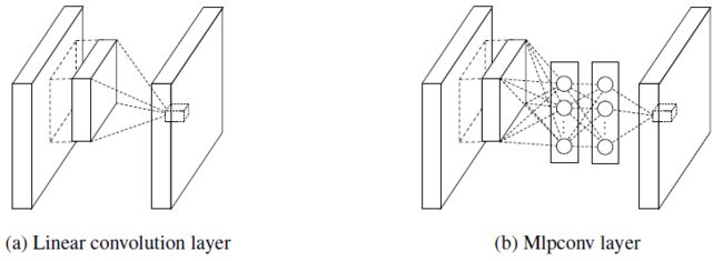
This paper suggests new type of layer called mlpconv, in which MLP replaces the GLM to convolve over the input. The reason to choose multilayer perceptron is

1. It is compatible with the structure of convolutional neural networks, which is trained using back-propagation.
2. It can e a deep model itself, which is consistent with the spirit of feature re-use.

Figure 1: Comparison of linear convolution layer and mlpconv layer.

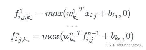
When nn is the number of layers in the multilayer perceptron, mlpconv layer can be calculated as follows:

 

1x1 Convolution

Mlpconv can be explained by a convolution layer with 1x1 convolution kernel. What the 1x1 convolution kernel does is:

1. It leads to dimension reductionality for the number of channel (e.g. an image of 100x100 with 30 features on convolution with 20 filters of 1x1 would result in size of 100x100x20.)
   • Comparison with pooling layer which reduce the height and width of the feature
2. It helps by adding non-linearity to the network in order to learn higher abstraction.
   • 1x1 filter calculate a linear combination of all corresponding pixels (neurons) of the input channels and output the result through an activation function which adds up the non-linearity.

 

Figure 2: Convolution with kernel of size 3x3 (left) vs. Convolution with kernel of size 1x1 (right)

Global Average Pooling

In conventional convolutional neural network, the feature maps of the last convolutional layer are vectorized and fed into fully connected layers followed by a softmax logistic regression layer.

Problem of the fully-connected layers:

• Prone to overfitting and heavily depend on dropout regularization
• Difficult to interpret how the category level information from the objective cost layer is passed back to the previous convolution layer

This paper propose a global average pooling (GAP) to replace the traditional fully connected layers in CNN. The idea is to generate one feature map for each corresponding category of the classification task in the last mlpconv layer. We take the average of each feature map, and the resulting vector is fed directly into the softmax layer.

Figure 3: Example of global average pooling (GAP)

Advantage of GAP over the fully-connected layers:

• It is more native to the convolution structure by enforcing correspondences between feature maps and categories.
  • Thus, the feature maps can be easily interpreted as categories confidence maps.
• There is no parameter to optimize in the global average pooling thus overfitting is avoided at this layer.
• It sums out the spatial information thus it is more robust to spatial translations of the input.

Network In Network Structure

As shown in Figure 4, the overall structure of NIN is a stack of mlpconv layers, on top of which lie the global average pooling and the objective cost layer. The number of layers in both NIN and the micro networks is flexible and can be tuned for specific tasks.

Figure 4: The overall structure of Network In Network. In this paper, the NINs include the stacking of three mlpconv layers and one global average pooling layer.

References

• Paper: Network In Network [Link]
• Blog: One by One Convolution - counter-intuitively useful [Link]
• Video: CNN16. Network in Network and 1*1 Convolutions by Andrew Ng [Link]