GAN史上最全基础入门总结
阅读提醒:中英文混杂
1. Introduction to GAN
1.1 Motivation
Generative models:
-
explicit models: Likelihood-based models ( autoregressive and flows/VAE)
-
implicit models: sample z → sample x, learning the deep neural network without explicit density estimation
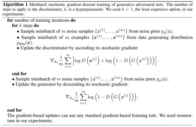
1.2 GAN (original GAN) [Goodfellow, NIPS, 2014]
G captures the data distribution, D estimates the divergence between p d a t a p_{data} pdata and p G p_G pG.
m i n G m a x D V ( G , D ) V ( G , D ) = E x ∼ p d a t a [ log D ( x ) ] + E z ∼ p z [ log ( 1 − D ( G ( z ) ) ) ] min_Gmax_D V(G,D) \\ V(G,D) = \mathbb{E}_{x\sim p_{data}}[\log D(x)] + \mathbb{E}_{z\sim p_{z}}[\log (1-D(G(z)))] minGmaxDV(G,D)V(G,D)=Ex∼pdata[logD(x)]+Ez∼pz[log(1−D(G(z)))]
D尽力区别原始数据与生成数据的区别,形成一个二分类器;G给D提供负样本,并且尽力期骗D使D犯错。
# last layer of D is nn.Sigmoid()
criterion=nn.BCELoss()
# Discriminator
f_loss = criterion(netD(fake_img.detach()), f_l)
r_loss = criterion(netD(real_img.detach()), r_l)
D_loss = (f_loss+r_loss)/2
# Generator
G_loss = criterion(netD(fake_img), r_l)  # 注意用的是real的label
Limitations:
- unstable convergence
- vanishing gradient
- more collapse
1.3 Evaluation
Parzen-Window density estimator (Kernel density estimator)
- 只适用于低维
- could be unreliable
Inception Score (IS)
I S ( x ) = exp ( H ( y ) − H ( y ∣ x ) ) IS(x) = \exp(H(y)-H(y|x)) IS(x)=exp(H(y)−H(y∣x))
- IS 越大越好:希望 H ( y ) H(y) H(y)越大越好,表明生成图片的种类越多;希望 H ( y ∣ x ) H(y|x) H(y∣x)越小越好,表明生成图片 x x x后其类别确定,即能够产生被分类的real image.
- IS 没有充分度量diversity
Frechet Inception Distance (FID)
- FID 越小越好
1.4 GAN theory
1.4.1 Bayes-Optimal Discriminator
用D衡量divergence,小的divergence是使discriminator很难分辨的东西,这个divergence不必显示表达,而是用一个NN来实现,这个NN就是D。
D ∗ = a r g m a x D V ( G , D ) D ∗ ( x ) = p d a t a ( x ) p d a t a ( x ) + p G ( x ) m a x V ( G , D ) = V ( G , D ∗ ) = − 2 log 2 + 2 J S D ( p d a t a ∣ ∣ p G ) G ∗ = a r g m i n G m a x D V ( G , D ) = a r g m i n G D i v ( p G , p d a t a ) D^*=argmax_DV(G,D) \\ D^*(x) = \frac{p_{data}(x)}{p_{data}(x)+p_{G}(x)}\\ max V(G,D) = V(G,D^*)=-2\log2+2JSD(p_{data}||p_G) \\ G^*=argmin_Gmax_D V(G,D) = argmin_G Div(p_G,p_{data}) D∗=argmaxDV(G,D)D∗(x)=pdata(x)+pG(x)pdata(x)maxV(G,D)=V(G,D∗)=−2log2+2JSD(pdata∣∣pG)G∗=argminGmaxDV(G,D)=argminGDiv(pG,pdata)
1.4.2 Mode collapse
Discriminator Saturation: G产生的图片被D highly confident认为是fake,因此G无法更新,因为梯度为0。
原论文措施:
- alternating optimization;
- non saturating formation: When training G, m i n E log ( 1 − D ( G ( z ) ) ) min \mathbb{E}\log(1-D(G(z))) minElog(1−D(G(z)))→ m a x E log D ( G ( z ) ) max \mathbb{E}\log D(G(z)) maxElogD(G(z))
2. GAN Progression
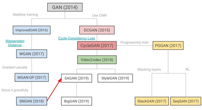
2.1 DCGAN (Deep Convolutional GAN) [Randford et al, 2016]
GAN框架在图片生成中的改进
- paper: https://arxiv.org/abs/1511.06434
Architecture design

- no pooling or fully connected layers;
- G使用transpose convolutions to do upsampling;
- G和D中使用batch normalization防止mode collapse, no BN in output of G and input of D;
- ReLU for G and LeakyReLU(0.2) for D;
- output layer: tanh for G and sigmoid for D
- preprocessing: 图片处理取值范围为[-1, 1]
Optimization details
Adam: lr = 2e-4, beta1=0.5, batch size=128
Results summary
- Incredible samples for any generative model
- GANs could be made to work well with architecture details
- Perceptually good samples and interpolations (bedrooms; faces)
- Representation Learning (CIFAR-10 classification task)
2.2 Improved Training of GANs [Salimans et al, 2016]
- paper: https://arxiv.org/abs/1606.03498
- github: https://github.com/openai/improved_gan
main ideas
- training tricks:
- Feature matching
- Minibatch discrimination: use side information, help address mode collapse
- Historical averaging
- One-sided label smoothing: for D not G
- Virtual batch normalization: reference batch
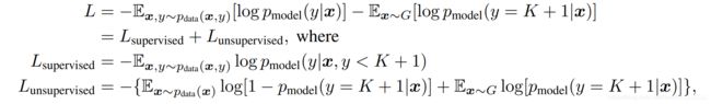
- semi-supervised learning: new loss function
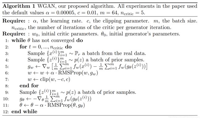
2.3 WGAN [Arjovsky et al, 2017]
- paper: https://arxiv.org/abs/1701.07875
- code reference: https://github.com/eriklindernoren/PyTorch-GAN/blob/master/implementations/wgan/wgan.py
提出用Earth Mover Distance衡量分布间的距离,希望用通过优化其对偶问题找到W,提出了用lipschitzness限制D然后进行优化。其优化方案是进行weight clipping,强制截断。尽管clipping不是一个好的方案,但是证明了这种对W的近似方法解决了JSD在训练的instability problem,让训练更加robust,减少mode collapse。
Summary
-
New divergence measure for optimizing the generator (Earth Mover Distance)
KaTeX parse error: No such environment: align at position 8: \begin{̲a̲l̲i̲g̲n̲}̲ W(\mathbb{P}_{…
优化W的对偶问题:
m i n G m a x D ∈ D E x ∼ P d a t a [ D ( x ) ] + E x ∼ P G [ D ( x ) ] min_G max_{D\in\mathscr{D}}\mathbb{E}_{x\sim~P_{data}}[D(x)] +\mathbb{E}_{x\sim~P_{G}}[D(x)] minGmaxD∈DEx∼ Pdata[D(x)]+Ex∼ PG[D(x)] -
Addresses instabilities with JSD version (sigmoid cross entropy)
-
Robust to architectural choices
-
Progress on mode collapse and stability of derivative wrt input
-
Introduces the idea of using lipschitzness to stabilize GAN training
Limitation
- weight clipping 不是解决lipschitzness问题的最好方式,很容易导致梯度消失或者梯度爆炸
WGAN与original GAN第一种形式相比,只改了四点:
- 判别器最后一层去掉sigmoid
- 生成器和判别器的loss不取log (因为使用了EM Distance)
- 每次更新判别器的参数之后把它们的绝对值截断到不超过一个固定常数c(weight clipping)
- 不要用基于动量的优化算法(包括momentum和Adam),推荐RMSProp,SGD也行
# 损失函数变化
D_loss = -torch.mean(netD(real_imgs.detach()))+torch.mean(netD(fake_imgs.detach()))
## weight clipping
for p in netD.parameters():
    # 限制大小
    p.data.clamp_(-c, c)

G_loss = -torch.mean(netD(fake_imgs.detach()))
2.4 Imporved WGAN [Gulrajani et al. 2017]
- github: https://github.com/igul222/improved_wgan_training
- paper: https://arxiv.org/abs/1704.00028
- code reference: https://github.com/eriklindernoren/PyTorch-GAN/tree/master/implementations/wgan
提出gradient penalty正则化项保证lipschitzness,训练更加robust,称为之后各种GAN的基本模型
m i n G m a x D ∈ D E x ∼ P d a t a [ D ( x ) ] + E x ∼ P G [ D ( x ) ] + λ E x ^ ∼ P x ^ [ ( ∇ x ^ ∣ ∣ D ( x ^ ) ∣ ∣ 2 − 1 ) 2 ] min_G max_{D\in\mathscr{D}}\mathbb{E}_{x\sim~P_{data}}[D(x)] +\mathbb{E}_{x\sim~P_{G}}[D(x)] + \lambda \mathbb{E}_{\hat{x}\sim~P_{\hat{x}}}[(\nabla_{\hat{x}}||D(\hat{x})||_2-1)^2] minGmaxD∈DEx∼ Pdata[D(x)]+Ex∼ PG[D(x)]+λEx^∼ Px^[(∇x^∣∣D(x^)∣∣2−1)2]

Architecture Detail
- no Batch Norm in Discriminator
Summary
- Robustness to architectural choices
- Became a very popular GAN model - 2000+ citations, has been used in NVIDIA’s Progressive GANs, StyleGAN, etc - biggest GAN successes
- Residual architecture widely adopted.
Limitation
- slow wall clock time due to gradient penalty.
- Gradient penalty applied on a heuristic distribution of samples from current generator. Could be unstable when learning rates are high.
# calculate Gradient Penalty
def compute_GP(discriminator, real_imgs, fake_imgs):
    epsilon = torch.Tensor(real_imgs.size(0),1,1,1).uniform_()
    x_hat = (epsilon * real_imgs + (1-epsilon) * fake_imgs).requires_grad_(True)
    outputs = discriminator(x_hat)
    gradients = autograd.grad(
        outputs = outputs,
        inputs = x_hat,
        create_graph=True,
        retain_graph=True,
        only_inputs=True
    )[0]
    gradients = gradiants.view(real_imgs.size(0), -1)
    gp = torch.mean((gradients.norm(2, dim=1)-1)**2)

    return gp

gradient_penalty = compute_GP(netD, img.data, fake_img.data)
D_loss = -torch.mean(netD(img.detach()) + torch.mean(netD(fake_img.detach())) + \
                     lambda_ * gradient_penalty    # 损失函数变化
2.5 SN-GAN (Spectral Normaliztion) [Miyato et al, ICLR, 2018]
- paper: https://arxiv.org/abs/1802.05957
- github: https://github.com/pfnet-research/sngan_projection
- github2: https://github.com/godisboy/SN-GAN
通过spectral norm谱范数约束discriminator每一层网络的权重矩阵W,以保证lipschitzness,增强了discriminator训练的稳定性。
keep gradient norm smaller than 1 everywhere.
spectral norm = largest singular value of W.
Because of heavy calculation of singular value of W, using power iteration method to estimate σ ( W ) \sigma(W) σ(W).
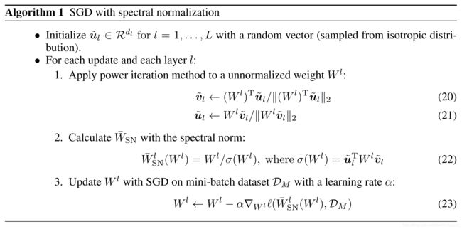
torch.nn.utils.spectral_norm: Spectral normalization stabilizes the training of discriminators (critics) in Generative Adversarial Networks (GANs) by rescaling the weight tensor with spectral norm σ of the weight matrix calculated using power iteration method.
summary
- High quality class conditional samples at Imagenet scale
- First GAN to work on full Imagenet (million image dataset)
- Computational benefits over WGAN-GP (single power iteration and no need of a backward pass)
2.6 SAGAN (Self-Attention GAN) [Zhang et al, 2018]
- paper: https://arxiv.org/abs/1805.08318
- github: https://github.com/heykeetae/Self-Attention-GAN
contributions
- Self-attention: consider Long-range dependency
- Spectral normalization (SN) for both G and D
- Imbalanced learning rate for G and D (TTUR)
2.7 Others
- BigGAN
- Based on SAGAN and SN
- Two to four times as many parameters
- Batch size * 8
- Truncation Trick
- Some insights about training stability
- StyleGAN
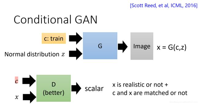
3. Creative conditional GAN / pix2pix
lots of applications:
- video2video (NVIDIA)
- GauGAN (NVIDIA)
- Learning to paint (GAN+RL)(Deepmind)
4. Unsupervised Conditional Generation-CycleGAN [ICCV, 2017]
- website: https://junyanz.github.io/CycleGAN/
- github: https://github.com/junyanz/pytorch-CycleGAN-and-pix2pix
learning to translate an image from a source domain X to a target domain Y in the absence of paired examples.
introduce cycle consistency.
[外链图片转存失败,源站可能有防盗链机制,建议将图片保存下来直接上传(img-rpyH0Pvz-1611629299630)(/pics/cycle.PNG)]
$$
L(G,F,D_X,D_Y)=L_{GAN}(G,D_Y,X,Y)+L_{GAN}(G,D_X,Y,X)+\lambda L_{cyc}(G,F) \
L_{GAN}(G,D_Y,X,Y) = \mathbb E_{y\sim p_{data}(y)}[\log D_Y(y)] + \mathbb E_{x\sim p_{data}(x)}[\log (1-D_Y(G(x))]\
L_{cyc}(G,F) = \mathbb E_{x\sim p_{data}(x)}[||F(G(x))-x||1] + \mathbb E{y\sim p_{data}(y)}[||G(F(y))-y||_1]
$$
5. Representations (Unsupervised Feature extraction)
5.1 InfoGAN (Information maximizing) [NIPs, 2016]
- paper: https://arxiv.org/abs/1606.03657
- github: https://github.com/openai/InfoGAN
learn disentangled representations in an unsupervised manner.
mutual information I ( c ; G ( z , c ) ) I(c;G(z,c)) I(c;G(z,c)) should be high→maximize lower bound of I = L I ( G , Q ) L_I(G,Q) LI(G,Q)
m i n G , Q m a x D V I n f o G A N ( D , G , Q ) = V ( D , G ) − λ L I ( G , Q ) L I ( G , Q ) = E x ∼ G ( z , c ) [ E c ′ ∼ P ( c ∣ x ) [ log Q ( c ′ ∣ x ) ] ] + H ( c ) ≤ I ( c ; G ( z , c ) ) min_{G,Q}max_DV_{InfoGAN}(D,G,Q)=V(D,G)-\lambda L_I(G,Q) \\ L_I(G,Q)=\mathbb{E}_{x\sim G(z,c)}[\mathbb{E}_{c'\sim P(c|x)}[\log Q(c'|x)]]+H(c) \le I(c;G(z,c)) minG,QmaxDVInfoGAN(D,G,Q)=V(D,G)−λLI(G,Q)LI(G,Q)=Ex∼G(z,c)[Ec′∼P(c∣x)[logQ(c′∣x)]]+H(c)≤I(c;G(z,c))
5.2 BiGAN and BigBiGAN
BiGAN [DeepMind, ICLR, 2017]
- paper: https://arxiv.org/abs/1605.09782v7
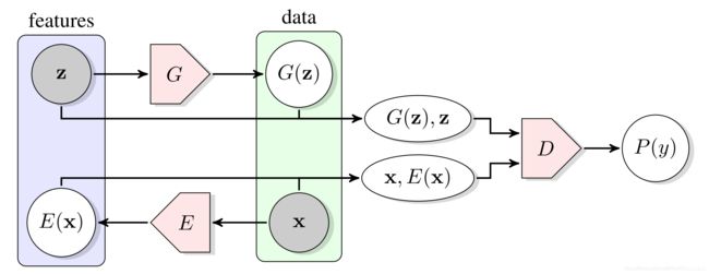
m i n G , E m a x D V ( D , E , G ) min_{G,E}max_DV(D,E,G) minG,EmaxDV(D,E,G)
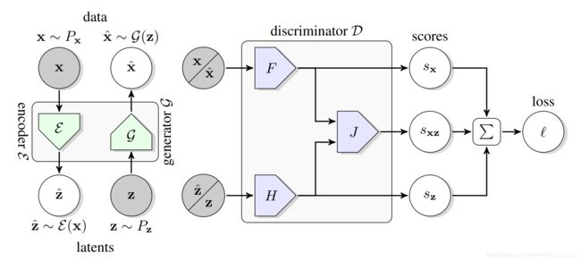
BigBiGAN [DeepMind, 2019]
- paper: https://arxiv.org/abs/1907.02544
References:
- CS294-158 spring2020(lecture 5-6)
- HongyiLi ML 2020(lesson 11)
- https://atcold.github.io/pytorch-Deep-Learning/en/week09/09-3/
- https://zhuanlan.zhihu.com/p/25071913