论文《Sequential Recommendation with Graph Neural Networks》阅读
论文《Sequential Recommendation with Graph Neural Networks》阅读
- 论文概况
- Introduction
- Method
-
- A.Interest Graph Construction
- B. Interest-fusion Graph Convolutional Layer
- C.Interest-extraction Graph Pooling Layer
- D. Prediction Layer
- 总结
论文概况
本文是2021年SIGIR上的一篇论文,该篇文章通过计算用户在会话中的主要兴趣并计算兴趣聚簇来解决顺序推荐问题
Introduction
作者提出了几个问题
- 并不是会话中的每个项目都能体现用户的兴趣,会话中夹杂大量噪音.
- 用户的喜好是迅速变化的,单从历史会话中很难捕获接下来的喜好变化
对于上述问题,作者提出SURGE网络(Sequential Recommendation with Graph Neural Networks):(1)从新角度解决顺序推荐,考虑隐信号行为和快速变化的偏好(2)通过物品-物品兴趣图,使用GNN网络将隐式信号转化为显式信号,设计动态池化来过滤和保留主要偏好以供推荐
Method
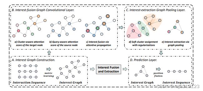
A.Interest Graph Construction
SURGE根据物品之间的相似度来构建兴趣图,一个会话中有n个物品,则有n*n的邻接矩阵,邻接矩阵的数值是按照相似度来计算,这里还使用了多头机制
M i j = cos ( w → ⊙ h ⃗ i , w → ⊙ h ⃗ j ) (1) M_{i j}=\cos \left(\overrightarrow{\mathbf{w}} \odot \vec{h}_{i}, \overrightarrow{\mathbf{w}} \odot \vec{h}_{j}\right)\tag{1} Mij=cos(w⊙hi,w⊙hj)(1)
M i j δ = cos ( w → δ ⊙ h ⃗ i , w → δ ⊙ h ⃗ j ) , M i j = 1 δ ∑ δ = 1 ϕ M i j δ (2) M_{i j}^{\delta}=\cos \left(\overrightarrow{\mathbf{w}}_{\delta} \odot \vec{h}_{i}, \overrightarrow{\mathbf{w}}_{\delta} \odot \vec{h}_{j}\right), \quad M_{i j}=\frac{1}{\delta} \sum_{\delta=1}^{\phi} M_{i j}^{\delta}\tag{2} Mijδ=cos(wδ⊙hi,wδ⊙hj),Mij=δ1δ=1∑ϕMijδ(2)
此时,邻接矩阵每个位置都有相似度数值,设相似度数值大于某一阈值,则将此处数值设为1,其余为0
A i j = { 1 , M i j > = Rank ε n 2 ( M ) 0 , otherwise; (3) A_{i j}=\left\{\begin{array}{ll} 1, & M_{i j}>=\operatorname{Rank}_{\varepsilon n^{2}}(M) \\ 0, & \text { otherwise; } \end{array}\right.\tag{3} Aij={1,0,Mij>=Rankεn2(M) otherwise; (3)
B. Interest-fusion Graph Convolutional Layer
通过兴趣图来计算每个节点的向量表征,aggregate可以是Mean,Sum, Max, GRU,这里使用Sum,并且同样利用多头机制
h ⃗ i ′ = σ ( W a ⋅ Aggregate ( E i j ∗ h ⃗ j ∣ j ∈ N i ) + h ⃗ i ) . (4) \vec{h}_{i}^{\prime}=\sigma\left(\mathbf{W}_{\mathbf{a}} \cdot \text { Aggregate }\left(E_{i j} * \vec{h}_{j} \mid j \in \mathcal{N}_{i}\right)+\vec{h}_{i}\right) \text {. }\tag{4} hi′=σ(Wa⋅ Aggregate (Eij∗hj∣j∈Ni)+hi). (4)
h i ′ → = ∥ δ = 1 ϕ σ ( W a δ ⋅ Aggregate ( E i j δ ∗ h ⃗ j ∣ j ∈ N i ) + h ⃗ i ) , (5) \overrightarrow{h_{i}^{\prime}}=\|_{\delta=1}^{\phi} \sigma\left(\mathbf{W}_{\mathbf{a}}^{\delta} \cdot \text { Aggregate }\left(E_{i j}^{\delta} * \vec{h}_{j} \mid j \in \mathcal{N}_{i}\right)+\vec{h}_{i}\right),\tag{5} hi′=∥δ=1ϕσ(Waδ⋅ Aggregate (Eijδ∗hj∣j∈Ni)+hi),(5)
之后是 E i j E_{i j} Eij计算,包含聚簇注意力和查询感知注意力
聚簇注意力代表当前节点与邻居节点的相似度, h ⃗ i c \vec{h}_{i_{c}} hic是k-hop内的邻居向量的平均值
α i = Attention c ( W c h ⃗ i ∥ h ⃗ i c ∥ W c h ⃗ i ⊙ h ⃗ i c ) (6) \alpha_{i}=\text { Attention }_{c}\left(\mathbf{W}_{\mathbf{c}} \vec{h}_{i}\left\|\vec{h}_{i_{c}}\right\| \mathbf{W}_{\mathbf{c}} \vec{h}_{i} \odot \vec{h}_{i_{c}}\right)\tag{6} αi= Attention c(Wchi∥∥∥hic∥∥∥Wchi⊙hic)(6)
查询感知注意力代表邻居节点和目标物品的相似度
β j = Attention q ( W q h ⃗ j ∥ h ⃗ t ∥ W q h ⃗ j ⊙ h ⃗ t ) (7) \beta_{j}=\text { Attention }_{q}\left(\mathbf{W}_{\mathbf{q}} \vec{h}_{j}\left\|\vec{h}_{t}\right\| \mathbf{W}_{\mathbf{q}} \vec{h}_{j} \odot \vec{h}_{t}\right)\tag{7} βj= Attention q(Wqhj∥∥∥ht∥∥∥Wqhj⊙ht)(7)
最终注意力计算如下:
E i j = softmax j ( α i + β j ) = exp ( α i + β j ) ∑ k ∈ N i exp ( α i + β k ) (8) E_{i j}=\operatorname{softmax}_{j}\left(\alpha_{i}+\beta_{j}\right)=\frac{\exp \left(\alpha_{i}+\beta_{j}\right)}{\sum_{k \in \mathcal{N}_{i}} \exp \left(\alpha_{i}+\beta_{k}\right)}\tag{8} Eij=softmaxj(αi+βj)=∑k∈Niexp(αi+βk)exp(αi+βj)(8)
C.Interest-extraction Graph Pooling Layer
我们将n个项目的表征用S矩阵分为m个类, γ \gamma_{} γ是经过softmax的查询感知注意力.
{ h ⃗ 1 ∗ , h ⃗ 2 ∗ , … , h ⃗ m ∗ } = S T { h ⃗ 1 ′ , h ⃗ 2 ′ , … , h ⃗ n ′ } (9) \left\{\vec{h}_{1}^{*}, \vec{h}_{2}^{*}, \ldots, \vec{h}_{m}^{*}\right\}=S^{T}\left\{\vec{h}_{1}^{\prime}, \vec{h}_{2}^{\prime}, \ldots, \vec{h}_{n}^{\prime}\right\}\tag{9} {h1∗,h2∗,…,hm∗}=ST{h1′,h2′,…,hn′}(9)
{ γ 1 ∗ , γ 2 ∗ , … , γ m ∗ } = S T { γ 1 , γ 2 , … , γ n } (10) \left\{\gamma_{1}^{*}, \gamma_{2}^{*}, \ldots, \gamma_{m}^{*}\right\}=S^{T}\left\{\gamma_{1}, \gamma_{2}, \ldots, \gamma_{n}\right\}\tag{10} {γ1∗,γ2∗,…,γm∗}=ST{γ1,γ2,…,γn}(10)
W p \mathbf{W}_{\mathrm{p}} Wp对应着m个分类,矩阵S每一行由邻居节点影响
S i : = softmax ( W p ⋅ Aggregate ( A i j ∗ h ⃗ j ′ ∣ j ∈ N i ) ) (11) S_{i:}=\operatorname{softmax}\left(\mathbf{W}_{\mathrm{p}} \cdot \text { Aggregate }\left(A_{i j} * \vec{h}_{j}^{\prime} \mid j \in \mathcal{N}_{i}\right)\right)\tag{11} Si:=softmax(Wp⋅ Aggregate (Aij∗hj′∣j∈Ni))(11)
同时,加入正则项来训练S
为了让相似的两个物品被分到同一类中,设:
L M = ∥ A , S S T ∥ F (12) L_{\mathrm{M}}=\left\|A, S S^{T}\right\|_{F}\tag{12} LM=∥∥A,SST∥∥F(12)
S S T S S^{T} SST代表两个点落入同一类的概率,在邻接矩阵中相连的点应被分为同一类
其次使用熵函数使得一个点尽可能只被分到一类中
L A = 1 n ∑ i = 1 n H ( S i : ) (13) L_{\mathrm{A}}=\frac{1}{n} \sum_{i=1}^{n} H\left(S_{i:}\right)\tag{13} LA=n1i=1∑nH(Si:)(13)
最后,保证当n个项目变成m个类时,类与类之间的时间关系可以与项目于项目之间的时间关系相同
L P = ∥ P n S , P m ∥ 2 (14) L_{\mathrm{P}}=\left\|P_{n} S, P_{m}\right\|_{2}\tag{14} LP=∥PnS,Pm∥2(14)
将所有项目的表征乘以分数加和,得到整体的用户兴趣
h ⃗ g = Readout ( { γ i ∗ h ⃗ i ′ , i ∈ G } ) , (15) \vec{h}_{g}=\operatorname{Readout}\left(\left\{\gamma_{i} * \vec{h}_{i}^{\prime}, i \in \mathcal{G}\right\}\right),\tag{15} hg=Readout({γi∗hi′,i∈G}),(15)
D. Prediction Layer
使用GRU来计算用户接下来可能感兴趣的项目类别
h ⃗ s = AUGRU ( { h ⃗ 1 ∗ , h ⃗ 2 ∗ , … , h ⃗ m ∗ } ) (16) \vec{h}_{s}=\operatorname{AUGRU}\left(\left\{\vec{h}_{1}^{*}, \vec{h}_{2}^{*}, \ldots, \vec{h}_{m}^{*}\right\}\right)\tag{16} hs=AUGRU({h1∗,h2∗,…,hm∗})(16)
进行用户点击物品预测,将目标项目 用户综合兴趣 用户预测兴趣类别相结合
y ^ = Predict ( h ⃗ s ∥ h ⃗ g ∥ h ⃗ t ∥ h ⃗ g ⊙ h ⃗ t ) (17) \hat{y}=\operatorname{Predict}\left(\vec{h}_{s}\left\|\vec{h}_{g}\right\| \vec{h}_{t} \| \vec{h}_{g} \odot \vec{h}_{t}\right)\tag{17} y^=Predict(hs∥∥∥hg∥∥∥ht∥hg⊙ht)(17)
使用交叉熵和正则项来训练参数

总结
SURGE使用了独特的兴趣图来进行GNN,同时还将项目聚类,通过RNN预测用户会点击的下一个物品类别,创新点值得借鉴.