深度学习图像处理目标检测图像分割计算机视觉 11--医疗影像分割
深度学习图像处理目标检测图像分割计算机视觉 11--医疗影像分割
- 摘要
- 一、医疗影像分割
- 二、U-Net
- 三、Brain Tumor Classification based on MR Images using GAN as a Pre-Trained Model基于 MR 图像的脑肿瘤分类使用 GAN 作为预训练模型
-
- 3.1、摘要
- 3.2、介绍
- 3.3、模型、结构
- 3.4、总结
摘要
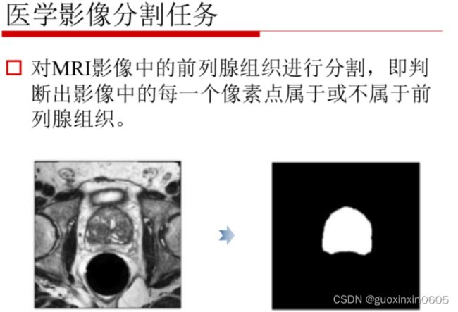
本周主要学习关于医疗影像分割的算法和例子,这里主要研究的是对MRI影像中的前列腺组织进行分割。对U-Net网络进行改进实现目标。学习一篇使用MRI图像的论文。毕设已经提交开题报告,在学习区块链内容。
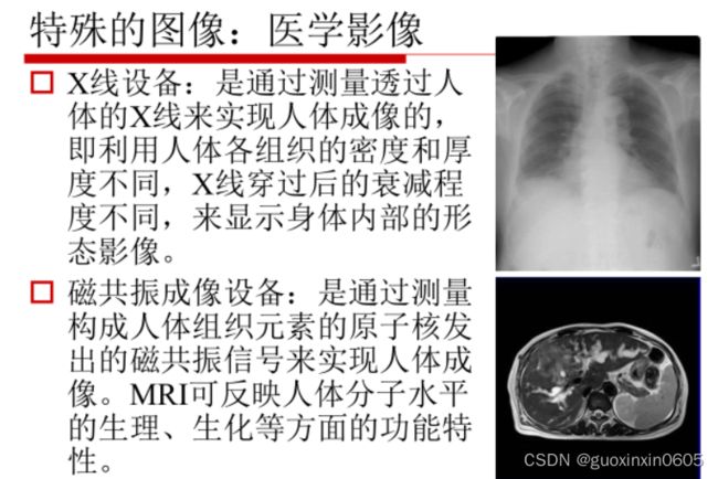
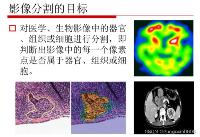
一、医疗影像分割


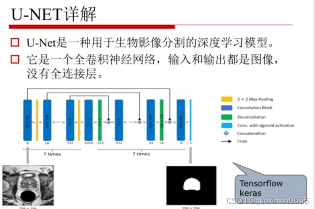


二、U-Net

import numpy as np # linear algebra
import pandas as pd # data processing, CSV file I/O (e.g. pd.read_csv)
import os
import numpy as np
import pandas as pd
import scipy.io
from skimage.transform import resize
import matplotlib.pyplot as plt
from tqdm import tqdm
import gc
gc.collect()

# Input data files are available in the "../input/" directory.
# For example, running this (by clicking run or pressing Shift+Enter) will list the files in the input directory

import os
print(os.listdir("../input"))


# https://www.kaggle.com/pierrenicolaspiquin/oct-segmentation/data
# Settings
input_path = os.path.join('..', 'input', '2015_boe_chiu', '2015_BOE_Chiu')
subject_path = [os.path.join(input_path, 'Subject_0{}.mat'.format(i)) for i in range(1, 10)] + [os.path.join(input_path, 'Subject_10.mat')]

data_indexes = [10, 15, 20, 25, 28, 30, 32, 35, 40, 45, 50]

width = 284
height = 284
width_out = 196
height_out = 196

mat = scipy.io.loadmat(subject_path[0])
img_tensor = mat['images']
manual_fluid_tensor_1 = mat['manualFluid1']

img_array = np.transpose(img_tensor, (2, 0, 1))
manual_fluid_array = np.transpose(manual_fluid_tensor_1, (2, 0, 1))


plt.imshow(img_array[25])
plt.imshow(manual_fluid_array[25])
def thresh(x):
    if x == 0:
        return 0
    else:
        return 1

thresh = np.vectorize(thresh, otypes=[np.float])

def create_dataset(paths):
    x = []
    y = []

    for path in tqdm(paths):
        mat = scipy.io.loadmat(path)
        img_tensor = mat['images']
        fluid_tensor = mat['manualFluid1']

        img_array = np.transpose(img_tensor, (2, 0 ,1)) / 255
        img_array = resize(img_array, (img_array.shape[0], width, height))
        fluid_array = np.transpose(fluid_tensor, (2, 0 ,1))
        fluid_array = thresh(fluid_array)
        fluid_array  = resize(fluid_array, (fluid_array .shape[0], width_out, height_out))

        for idx in data_indexes:
            x += [np.expand_dims(img_array[idx], 0)]
            y += [np.expand_dims(fluid_array[idx], 0)]
    return np.array(x), np.array(y)

x_train, y_train = create_dataset(subject_path[:9])
x_val, y_val = create_dataset(subject_path[9:])

x_train.shape, y_train.shape, x_val.shape, y_val.shape


import torch
import torchvision
import torch.nn as nn
import torch.nn.functional as F
import torch.optim as optim
from torch.autograd import Variable
from tqdm import trange
from time import sleep
use_gpu = torch.cuda.is_available()


batch_size = 9
epochs = 1000
epoch_lapse = 50
threshold = 0.5
sample_size = None


class UNet(nn.Module):
    def contracting_block(self, in_channels, out_channels, kernel_size=3):
        block = torch.nn.Sequential(
                    torch.nn.Conv2d(kernel_size=kernel_size, in_channels=in_channels, out_channels=out_channels),
                    torch.nn.ReLU(),
                    torch.nn.BatchNorm2d(out_channels),
                    torch.nn.Conv2d(kernel_size=kernel_size, in_channels=out_channels, out_channels=out_channels),
                    torch.nn.ReLU(),
                    torch.nn.BatchNorm2d(out_channels),
                )
        return block

    def expansive_block(self, in_channels, mid_channel, out_channels, kernel_size=3):
            block = torch.nn.Sequential(
                    torch.nn.Conv2d(kernel_size=kernel_size, in_channels=in_channels, out_channels=mid_channel),
                    torch.nn.ReLU(),
                    torch.nn.BatchNorm2d(mid_channel),
                    torch.nn.Conv2d(kernel_size=kernel_size, in_channels=mid_channel, out_channels=mid_channel),
                    torch.nn.ReLU(),
                    torch.nn.BatchNorm2d(mid_channel),
                    torch.nn.ConvTranspose2d(in_channels=mid_channel, out_channels=out_channels, kernel_size=3, stride=2, padding=1, output_padding=1)
                    )
            return  block

    def final_block(self, in_channels, mid_channel, out_channels, kernel_size=3):
            block = torch.nn.Sequential(
                    torch.nn.Conv2d(kernel_size=kernel_size, in_channels=in_channels, out_channels=mid_channel),
                    torch.nn.ReLU(),
                    torch.nn.BatchNorm2d(mid_channel),
                    torch.nn.Conv2d(kernel_size=kernel_size, in_channels=mid_channel, out_channels=mid_channel),
                    torch.nn.ReLU(),
                    torch.nn.BatchNorm2d(mid_channel),
                    torch.nn.Conv2d(kernel_size=kernel_size, in_channels=mid_channel, out_channels=out_channels, padding=1),
                    torch.nn.ReLU(),
                    torch.nn.BatchNorm2d(out_channels),
                    )
            return  block

    def __init__(self, in_channel, out_channel):
        super(UNet, self).__init__()
        #Encode
        self.conv_encode1 = self.contracting_block(in_channels=in_channel, out_channels=64)
        self.conv_maxpool1 = torch.nn.MaxPool2d(kernel_size=2)
        self.conv_encode2 = self.contracting_block(64, 128)
        self.conv_maxpool2 = torch.nn.MaxPool2d(kernel_size=2)
        self.conv_encode3 = self.contracting_block(128, 256)
        self.conv_maxpool3 = torch.nn.MaxPool2d(kernel_size=2)
        # Bottleneck
        self.bottleneck = torch.nn.Sequential(
                            torch.nn.Conv2d(kernel_size=3, in_channels=256, out_channels=512),
                            torch.nn.ReLU(),
                            torch.nn.BatchNorm2d(512),
                            torch.nn.Conv2d(kernel_size=3, in_channels=512, out_channels=512),
                            torch.nn.ReLU(),
                            torch.nn.BatchNorm2d(512),
                            torch.nn.ConvTranspose2d(in_channels=512, out_channels=256, kernel_size=3, stride=2, padding=1, output_padding=1)
                            )
        # Decode
        self.conv_decode3 = self.expansive_block(512, 256, 128)
        self.conv_decode2 = self.expansive_block(256, 128, 64)
        self.final_layer = self.final_block(128, 64, out_channel)

    def crop_and_concat(self, upsampled, bypass, crop=False):
        if crop:
            c = (bypass.size()[2] - upsampled.size()[2]) // 2
            bypass = F.pad(bypass, (-c, -c, -c, -c))
        return torch.cat((upsampled, bypass), 1)

    def forward(self, x):
        # Encode
        encode_block1 = self.conv_encode1(x)
        encode_pool1 = self.conv_maxpool1(encode_block1)
        encode_block2 = self.conv_encode2(encode_pool1)
        encode_pool2 = self.conv_maxpool2(encode_block2)
        encode_block3 = self.conv_encode3(encode_pool2)
        encode_pool3 = self.conv_maxpool3(encode_block3)
        # Bottleneck
        bottleneck1 = self.bottleneck(encode_pool3)
        # Decode
        ##print(x.shape, encode_block1.shape, encode_block2.shape, encode_block3.shape, bottleneck1.shape)
        ##print('Decode Block 3')
        ##print(bottleneck1.shape, encode_block3.shape)
        decode_block3 = self.crop_and_concat(bottleneck1, encode_block3, crop=True)
        ##print(decode_block3.shape)
        ##print('Decode Block 2')
        cat_layer2 = self.conv_decode3(decode_block3)
        ##print(cat_layer2.shape, encode_block2.shape)
        decode_block2 = self.crop_and_concat(cat_layer2, encode_block2, crop=True)
        cat_layer1 = self.conv_decode2(decode_block2)
        ##print(cat_layer1.shape, encode_block1.shape)
        ##print('Final Layer')
        ##print(cat_layer1.shape, encode_block1.shape)
        decode_block1 = self.crop_and_concat(cat_layer1, encode_block1, crop=True)
        ##print(decode_block1.shape)
        final_layer = self.final_layer(decode_block1)
        ##print(final_layer.shape)
        return  final_layer


def train_step(inputs, labels, optimizer, criterion):
    optimizer.zero_grad()
    # forward + backward + optimize
    outputs = unet(inputs)
    # outputs.shape =(batch_size, n_classes, img_cols, img_rows)
    outputs = outputs.permute(0, 2, 3, 1)
    # outputs.shape =(batch_size, img_cols, img_rows, n_classes)
    outputs = outputs.resize(batch_size*width_out*height_out, 2)
    labels = labels.resize(batch_size*width_out*height_out)
    loss = criterion(outputs, labels)
    loss.backward()
    optimizer.step()
    return loss

learning_rate = 0.01
unet = UNet(in_channel=1,out_channel=2)
if use_gpu:
    unet = unet.cuda()
criterion = nn.CrossEntropyLoss()
optimizer = optim.SGD(unet.parameters(), lr = 0.01, momentum=0.99)

def get_val_loss(x_val, y_val):
    x_val = torch.from_numpy(x_val).float()
    y_val = torch.from_numpy(y_val).long()
    if use_gpu:
        x_val = x_val.cuda()
        y_val = y_val.cuda()
    m = x_val.shape[0]
    outputs = unet(x_val)
    # outputs.shape =(batch_size, n_classes, img_cols, img_rows)
    outputs = outputs.permute(0, 2, 3, 1)
    # outputs.shape =(batch_size, img_cols, img_rows, n_classes)
    outputs = outputs.resize(m*width_out*height_out, 2)
    labels = y_val.resize(m*width_out*height_out)
    loss = F.cross_entropy(outputs, labels)
    return loss.data

epoch_iter = np.ceil(x_train.shape[0] / batch_size).astype(int)
t = trange(epochs, leave=True)
for _ in t:
    total_loss = 0
    for i in range(epoch_iter):
        batch_train_x = torch.from_numpy(x_train[i * batch_size : (i + 1) * batch_size]).float()
        batch_train_y = torch.from_numpy(y_train[i * batch_size : (i + 1) * batch_size]).long()
        if use_gpu:
            batch_train_x = batch_train_x.cuda()
            batch_train_y = batch_train_y.cuda()
        batch_loss = train_step(batch_train_x , batch_train_y, optimizer, criterion)
        total_loss += batch_loss
    if (_+1) % epoch_lapse == 0:
        val_loss = get_val_loss(x_val, y_val)
        print(f"Total loss in epoch {_+1} : {total_loss / epoch_iter} and validation loss : {val_loss}")

gc.collect()
def plot_examples(datax, datay, num_examples=3):
    fig, ax = plt.subplots(nrows=3, ncols=4, figsize=(18,4*num_examples))
    m = datax.shape[0]
    for row_num in range(num_examples):
        image_indx = np.random.randint(m)
        image_arr = unet(torch.from_numpy(datax[image_indx:image_indx+1]).float().cuda()).squeeze(0).detach().cpu().numpy()
        ax[row_num][0].imshow(np.transpose(datax[image_indx], (1,2,0))[:,:,0])
        ax[row_num][0].set_title("Orignal Image")
        ax[row_num][1].imshow(np.transpose(image_arr, (1,2,0))[:,:,0])
        ax[row_num][1].set_title("Segmented Image")
        ax[row_num][2].imshow(image_arr.argmax(0))
        ax[row_num][2].set_title("Segmented Image localization")
        ax[row_num][3].imshow(np.transpose(datay[image_indx], (1,2,0))[:,:,0])
        ax[row_num][3].set_title("Target image")
    plt.show()

plot_examples(x_train, y_train)

三、Brain Tumor Classification based on MR Images using GAN as a Pre-Trained Model基于 MR 图像的脑肿瘤分类使用 GAN 作为预训练模型
3.1、摘要
在医疗行业中,疾病误诊是公认的最常见和最有害的医疗错误,它可能以生命为代价。放射科医生需要大量的时间来手动注释和分割图像。近年来,深度学习在计算机视觉领域发挥着至关重要的作用。它在医疗行业的一个关键用途是最小化误诊和标注和分割图像所花费的时间。本文介绍了一种新的基于深度学习的MRI图像脑肿瘤分类方法。在生成对抗网络(generative adversarial network, GAN)中预先训练深度神经网络作为鉴别器,利用多尺度梯度GAN (multiscale gradient GAN, MSGGAN)进行辅助分类,提取特征并对图像进行分类。在鉴别器中,一个全连接块作为辅助分类器,另一个全连接块作为对抗器。完全连接的辅助块层被微调以区分肿瘤类型。提出的方法在两个公开可用的MRI数据集作为一个整体进行测试,这些数据集包括四种类型的脑 肿瘤(胶质瘤、脑膜瘤、垂体和无肿瘤)。该方法的准确度为98.57%,优于现有的方法。此外,当医学图像的可用性有限时,我们的方法似乎是一种有用的技术。
3.2、介绍
放射科医生使用两种方法对脑瘤进行分类。一种方法是确定给定的脑MR图像是正常的还是异常的,另一种方法是将异常的脑MR图像分类为不同的肿瘤类型。对于大量的MRI数据,手工进行脑肿瘤分类效率低,耗时长。为了解决这个问题,放射科医生可以使用自动分类来识别最小介入的脑肿瘤MR图像。
各种医学成像技术中,磁共振成像MRI是应用最广泛的技术。在MRI采集过程中,每次扫描提供大约150片(可能因设备不同而不同)的2D图像,以在没有电离辐射[3]的情况下,用高软组织对比度表示3D脑体积
3.3、模型、结构
该体系结构基于MSG-GAN(多尺度梯度)体系[8],并结合ACGAN论文[6]启发的辅助分类训练。我们的氮化镓架构和其他氮化镓架构一样,由两大神经网络组成:生成器和鉴别器。
生成器结构
待生成图像的潜在向量和标签是生成器所需的输入。将潜向量与标签相乘并发送到嵌入层,在训练过程中,当潜向量与它相乘(已标记的潜向量)时,嵌入层从潜向量学习标签表示。然后将嵌入层的输出传输到Conv 2d转置层,该层执行“反卷积”并从潜在向量生成4x4图像。然后根据选择的深度,提高图像分辨率(4x4->8x8->16x16->等),将图像传输到N个上采样和卷积块,生成图像。最后,将生成指定类的高分辨率图像。

鉴别器结构
发生器的输出,它是馈入鉴别器的图像。使用卷积块和平均池化,图像每一步向下采样2。在那之后,它通过一个小批量标准偏差运行。在这一步中,计算激活图中每个特征的标准偏差,然后在小批处理中取平均值。这种新的激活产生了地图。这些新的激活图被添加到鉴别器网络的末端。Mini-batch standard deviation的输出被输入到一个卷积块中,然后该卷积块被并行地(即分别地)转移到两个全连接块中。其中一个全连接块作为辅助分类器,决定输入图像属于哪一类;另一个全连接块作为对抗分类器,决定图像是真还是假

由于鉴别器已经学习了大脑和脑肿瘤的必要特征,网络的各层可以用于特征提取/迁移学习。在我们的微调过程中,我们冻结了所有的特征提取层(因为它们有GAN预先训练的权值,擅长特征提取),只使用训练数据和验证数据对辅助块的全连接层进行训练/微调。辅助块的初始全连接层由单个线性层组成,输出代表类的4个神经元。为了进行微调,在辅助块中的单一线性层之前,我们添加了另一个512单位的线性层。用亚当作为学习率0.001或4e-5的优化器,和交叉熵损失函数,
3.4、总结
在本文中,我们提出了一种利用GAN作为预训练模型从MR图像中分类脑肿瘤的新方法。我们使用公开可用的脑MRI数据集评估了它的性能。我们的结果表明,提出的前训练方法显著提高了整体效率。此外,当数据的可用性有限时,这种技术也很有用,可以应用于各种图像分类任务。我们将我们的结果与之前使用相同数据集的工作进行了比较。该方法在脑肿瘤MRI图像分类中准确率最高,为98.57%。
作为未来的工作,我们将改进我们的体系结构,以生成更真实的高分辨率MRI图像,这将有助于增加数据集的大小和解决数据集不平衡的问题。此外,我们将在未来测试我们的方法的效率以及对其他医学图像的改进。