线性回归法
1.简单线性回归
线性回归法跟我们在上一章所介绍的knn算法不同,knn算法主要用于解决分类问题,而线性回归算法则主要用于解决回归问题,对于现象回归算法来说,它也是思想非常简单,而且实现起来会非常容易,这里的实现容易,和他背后具有非常强的数学性质是相关的。那么这个相应的数学推导会稍微复杂一点,但也并不是特别难,但是由于有这种数学的支撑,使得我们的计算机的实现是很容易的。与此同时,线性回归法虽然非常简单,但是我们后面就会看到它是许多更加强大的非线性模型的基础,无论是多项式回归,逻辑回归甚至是svm,从某种程度上来讲都可以理解成是线性回归算法的一种。最重要的是线性回归算法,它可以得到的结果是具有非常好的可解释性的,也就是说我们能通过线性回归算法,通过对数据的分析模型的建立,学习到真实世界真正的知识。也正是因为如此,在很多学界领域的研究中,很多时候都会先尝试使用线性回归算法这样一个最基本,最简单的方式的。首先我们来看一下什么是先行回归算法,现象回归算法整体是这样的,在坐标平面上,相应的,每一个点都表示一个数据,假设是房产的价格的数据。

其中,横轴代表房屋的面积,纵轴代表房屋的价格,对于每一个房屋来说,就表示成每一个点,每一个房屋有自己的房屋的面积,同时有自己的价格,于是就可以在这个二维平面里形成一个点。那么,线性回归算法说,我们认为房屋的面积和价格之间呈一定的线性关系,也就是说随着房屋面积的增大。价格也会增大,并且这个增大的趋势是现行的,没有指数级的增大那么夸张。那么,在这样的一种假设下,我们就在想,我们可不可以找到这样的一条直线。我们希望这条直线可以最大程度的拟合这个样本特征和样本输出标记之间的关系。在我们这张图示的例子中,每一个样本只有一个特征,这个特征就是房屋的面积。而每一个样本的输出标记就是它的价格。
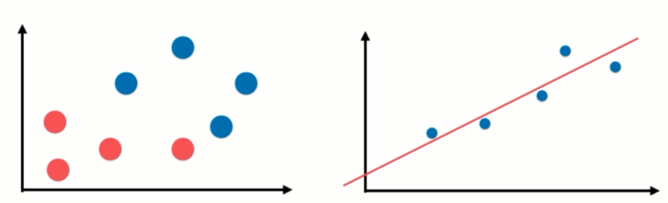
但是现在的这个二维平面图。跟分类问题的时候,那个二维平面图有很大的区别,分类问题,横轴和纵轴都是样本的特征,也就是说每一个点有两个样本特征。那么,这个样本的输出标记是被这个点是蓝色的点还是红色的点所表示的?蓝色的点代表它是恶性肿瘤,红色的点代表它是良性肿瘤。但是我们在这个例子中,只有横轴是样本的特征,就是房屋的面积,纵轴就已经是样本的输出标记了,也就是房屋的价格。这是因为在回归问题中,我们真正要预测的是一个具体的数值,这个具体的数值是在一个连续的空间里的,而不是可以简单的用不同的颜色来代表不同的类别,所以它需要占用一个坐标轴的位置。如果我们要想看有两个样本特征的回归问题的话就需要在三维空间中进行观察了。
对于这种样本的特征只有一个,这种情况使用线性回归法进行预测可以用简单线性回归这样的方法来称呼它,那么简单线性回归顾名思义它相对来说是更加简单的,我们通过对简单线性回归的学习,其实可以学习到线性回归算法相应的很多内容。之后我们再将它推广到样本特征有多个,样本特征有多个的时候,就叫做多元线性回归。
现在我们首先来看这个简单线性回归问题,那么我们说,我们想要找一条直线,这条直线最大程度的你和我的这些样本的特征点
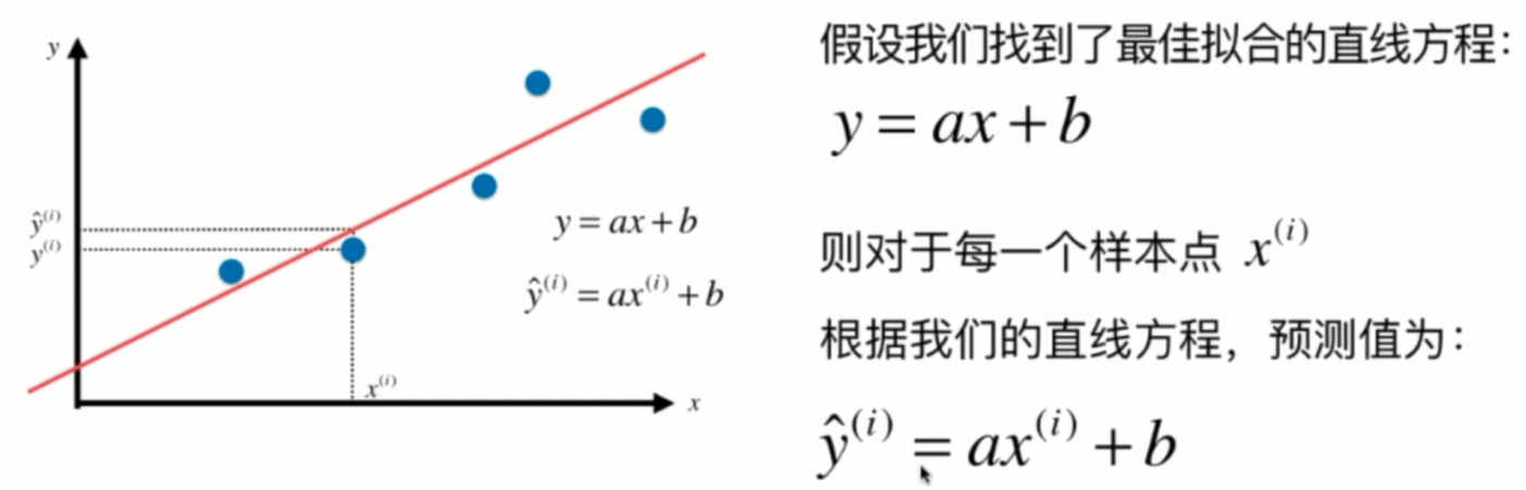
对于每一个点来说,它就对应一个。样本特征xi这里头这个i表示我们有多个数据点,它是第i个这个样本所对应的数据点。那么,相应的,它对应的这个输出标记就是yi,那么如果对于这条直线,我们把它的a和b找到了的话。那么相应的,我们就可以将xi这个特征值给带进这个方程中,用a去乘以xi再加上b,得到的这个值其实就是我们使用简单线性回归法预测出来的对于xi对应的这个特征,也就是对于xi这个房屋的面积,那么它的价格是多少。相应的,我们的预测值和真值之间就会有一个差距。
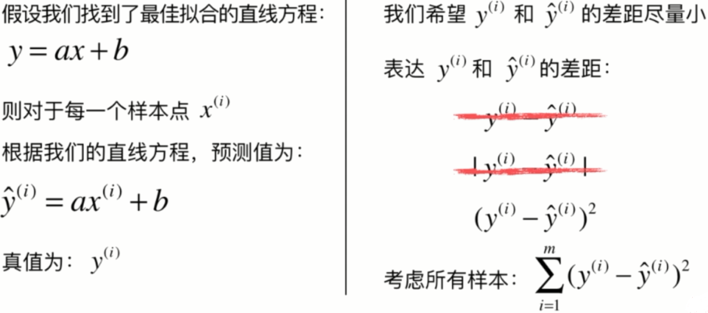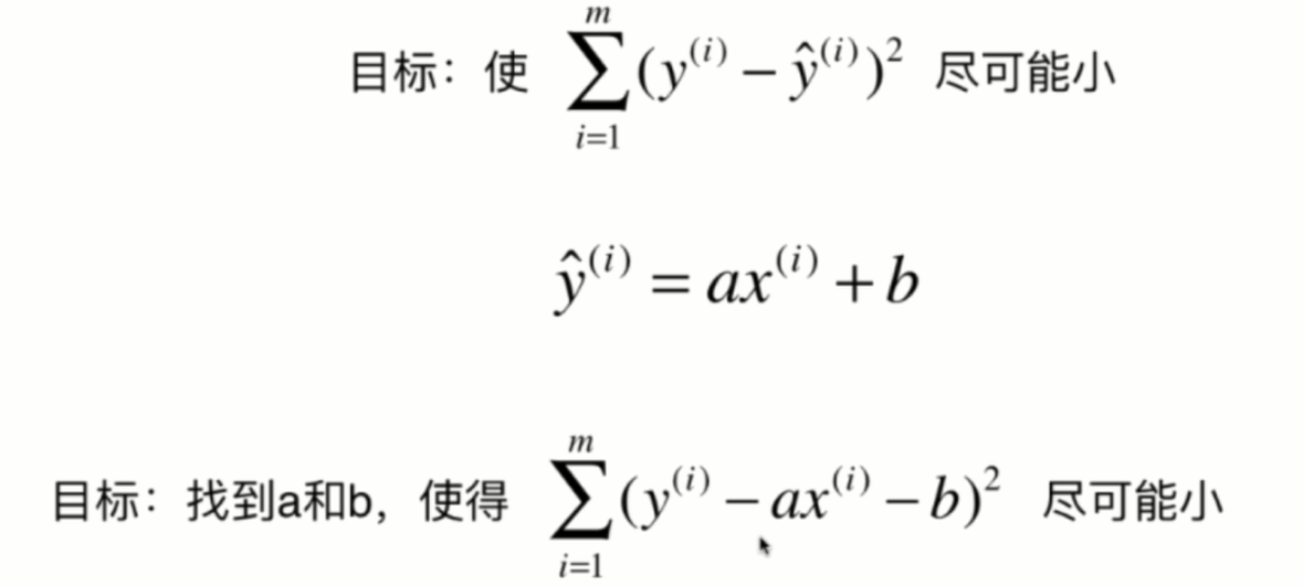
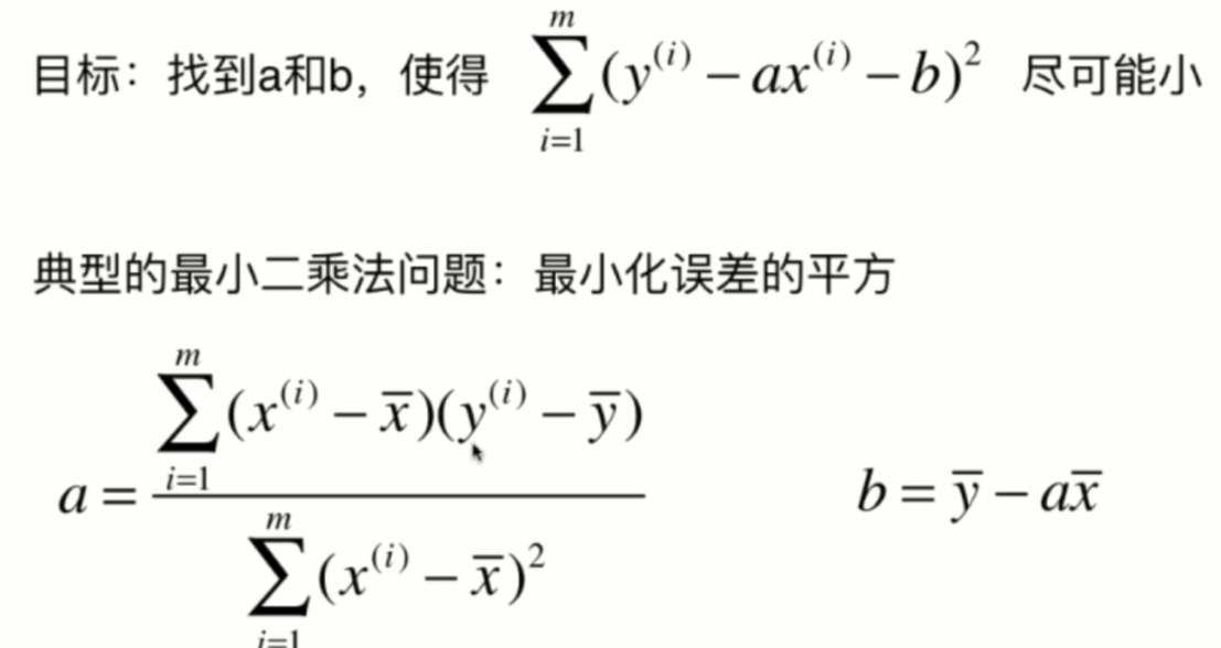
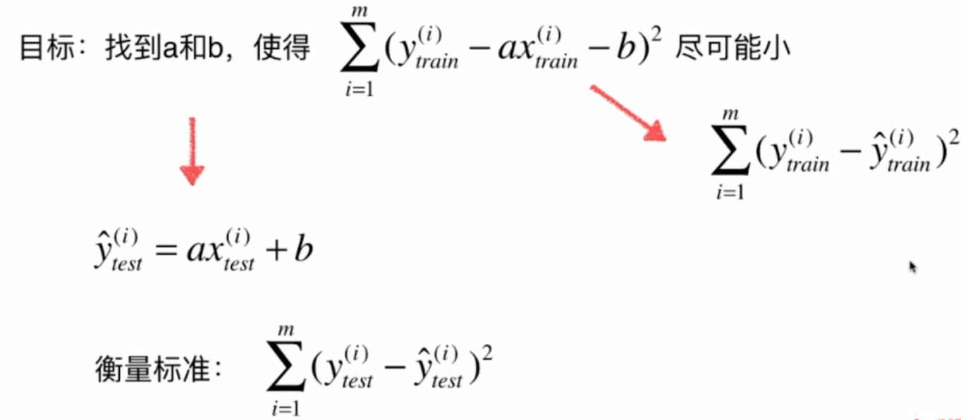
我们到这里推导出来的这个目标就是找到某一些参数值,使得某一个函数它尽可能的小,这是典型的一种机器学习算法的推导思路。换句话说,我们所谓的建模的过程其实就是找到一个模型最大程度的拟合的数据,那么在线性回归算法中,这个模型就是一个直线方程。
那么,所谓的最大拟合的数据,其实本质是找到这样的一个函数。在这里,我们称这个函数叫做损失函数,就是所谓的lost方式,也就是说,度量出我们的这个模型,没有拟合住的样本的这一部分,也就是损失的那一部分。但是呢,在有的算法中,有可能不良的是拟合的程度,那么在这种情况下呢,称这个函数为效用函数。那么,不管是损失函数还是效用函数,我们的机器学习算法都是通过分析问题确定问题的这种损失函数或者是效用函数。有的时候呢,我们将它统称为是一个目标函数,然后我们要做的事情就是最优化这个目标函数。那么,对于损失函数来说,我们希望让它尽可能的小,而对于效用函数来说,我们希望它尽可能的大。
当我们解决了这个最优化的问题之后,我们就获得了一个机器学习的模型。可以说所有的参数学习的算法都是这样的一个套路。所谓的参数学习算法就是我们要创建一个模型。而机器学习的任务就是要学习这些模型的参数,所谓的学习这些模型的参数。就是找到相应的这些参数,使得我们可以最优化我们的损失函数,或者是效应函数。很多算法都是如此,线性回归算法,多项式回归,逻辑回归,svm神经网络,他们的本质其实都是在学习相应的参数来最优化他们的目标函数,区别在于他们的模型不同,建立的这个目标函数是不同的,优化的方式也是不同的。
正是因为机器学期中大部分的算法都拥有这样的一个思路,所以有一个学科非常的重要,叫做最优化原理。实际上,最优化原理绝对不仅仅是机器学习算法中使用的一个思路,在经典的传统的计算机算法领域,最优化原理也发挥着重要的作用。我们使用计算机解决的非常多的问题,他们的本质其实都是一个最优化问题。比如说,我们对最短的路径感兴趣,对最小的生成数感兴趣,我们求解背包问题是希望背包的总价值是最大的等等。那么,对于这些传统的算法,他们背后的思想其实抽象出来也都可以在最优化原理这个领域中找到相关的答案。那么相应的,在最优化的原理领域还有一个分支领域,叫做凸优化,它解决的是一类特殊的优化问题。
2.最小二乘法

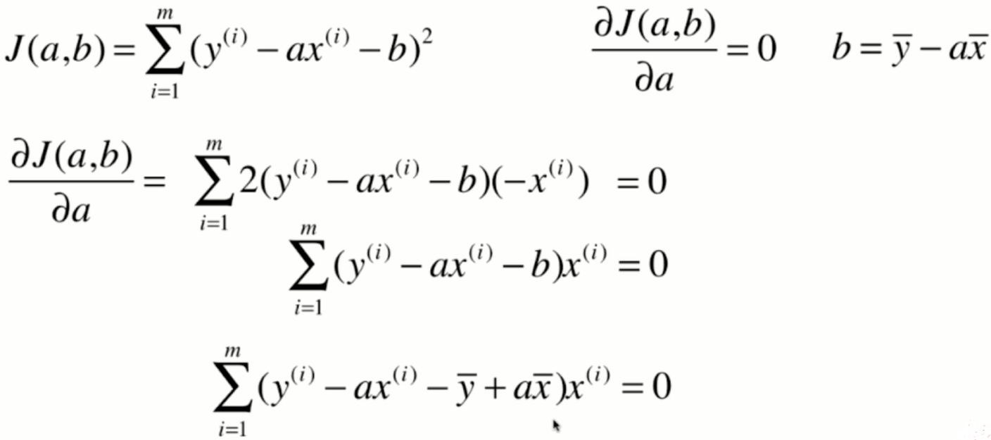
对于这个式子来说,a和b是我们的未知数,而不是xy,可能在初中和高中数学中比较习惯x和y是未知数,但是在我们的这个式子中,x和y是监督学习提供给的已知的信息,而a和b是我们真正要找的要求的这个参数。那么,在数学上,很多时候我们都用这种大g的方式来表示损失函数。想求这个损失函数的最小值,其实就是求一个函数的极值问题,求函数集植的一个最基本的方法,就是对这个函数的各个位置分量求导,让它的导数等于0,那么在导数等于0的地方,就是函数极值的地方


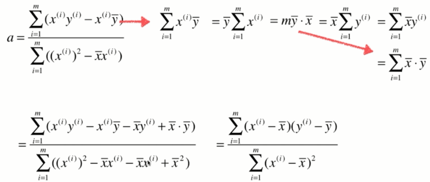
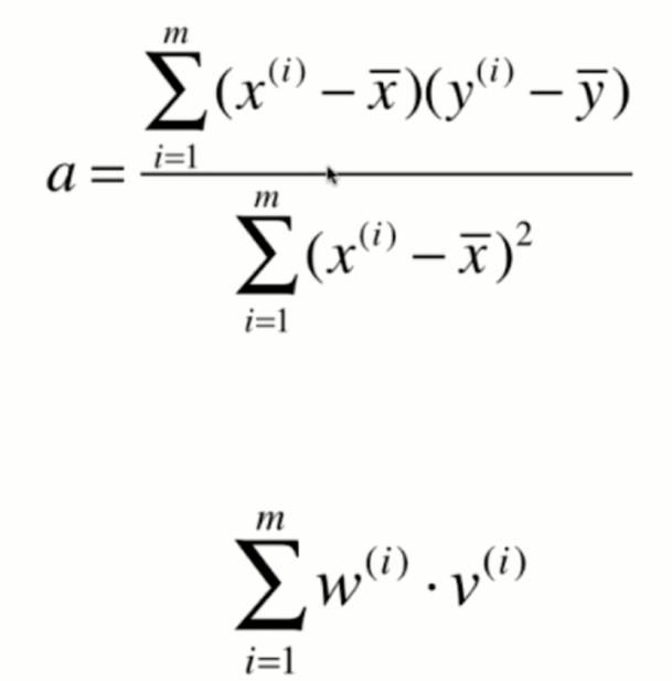
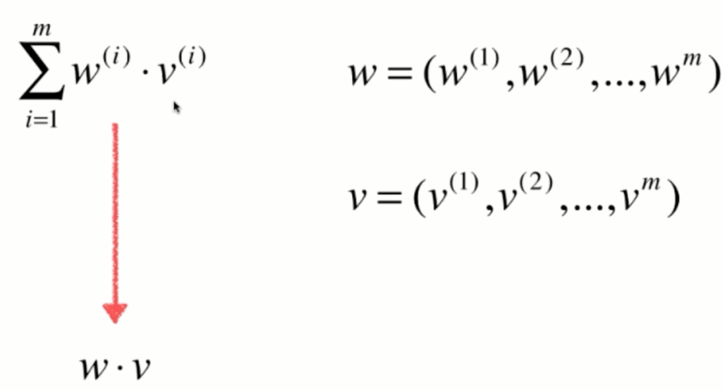
那么其实对于我们的最小二乘法来说,这个a就已经是我们最终的结果了,如果我们编程的话,我们直接按照这个式子去计算a就已经完全没有问题了。不过我们将这个柿子再进行一下整理,会得到一个更加简洁的表达式,而对于这个更加简洁的表达式可以在编程的时候使用一些技效加速它的计算过程。
3. 简单线性回归的实现
import numpy as np
import matplotlib.pyplot as plt
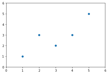
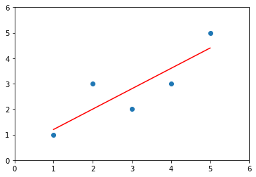
x = np.array([1., 2., 3., 4., 5.])
y = np.array([1., 3., 2., 3., 5.])
plt.scatter(x, y)
plt.axis([0, 6, 0, 6])
plt.show()
x_mean = np.mean(x)
y_mean = np.mean(y)
num = 0.0
d = 0.0
for x_i, y_i in zip(x, y):
    num += (x_i - x_mean) * (y_i - y_mean)
    d += (x_i - x_mean) ** 2

a = num/d
b = y_mean - a * x_mean
y_hat = a * x + b
plt.scatter(x, y)
plt.plot(x, y_hat, color='r')
plt.axis([0, 6, 0, 6])
plt.show()
x_predict = 6
y_predict = a * x_predict + b
y_predict
输出 5.2
import numpy as np


class SimpleLinearRegression1:

    def __init__(self):
        """初始化Simple Linear Regression 模型"""
        self.a_ = None
        self.b_ = None

    def fit(self, x_train, y_train):
        """根据训练数据集x_train,y_train训练Simple Linear Regression模型"""
        assert x_train.ndim == 1, \
            "Simple Linear Regressor can only solve single feature training data."
        assert len(x_train) == len(y_train), \
            "the size of x_train must be equal to the size of y_train"

        x_mean = np.mean(x_train)
        y_mean = np.mean(y_train)

        num = 0.0
        d = 0.0
        for x, y in zip(x_train, y_train):
            num += (x - x_mean) * (y - y_mean)
            d += (x - x_mean) ** 2

        self.a_ = num / d
        self.b_ = y_mean - self.a_ * x_mean

        return self

    def predict(self, x_predict):
        """给定待预测数据集x_predict,返回表示x_predict的结果向量"""
        assert x_predict.ndim == 1, \
            "Simple Linear Regressor can only solve single feature training data."
        assert self.a_ is not None and self.b_ is not None, \
            "must fit before predict!"

        return np.array([self._predict(x) for x in x_predict])

    def _predict(self, x_single):
        """给定单个待预测数据x,返回x的预测结果值"""
        return self.a_ * x_single + self.b_

    def __repr__(self):
        return "SimpleLinearRegression1()"
4.向量化
class SimpleLinearRegression2:

    def __init__(self):
        """初始化Simple Linear Regression模型"""
        self.a_ = None
        self.b_ = None

    def fit(self, x_train, y_train):
        """根据训练数据集x_train,y_train训练Simple Linear Regression模型"""
        assert x_train.ndim == 1, \
            "Simple Linear Regressor can only solve single feature training data."
        assert len(x_train) == len(y_train), \
            "the size of x_train must be equal to the size of y_train"

        x_mean = np.mean(x_train)
        y_mean = np.mean(y_train)

        self.a_ = (x_train - x_mean).dot(y_train - y_mean) / (x_train - x_mean).dot(x_train - x_mean)
        self.b_ = y_mean - self.a_ * x_mean

        return self

    def predict(self, x_predict):
        """给定待预测数据集x_predict,返回表示x_predict的结果向量"""
        assert x_predict.ndim == 1, \
            "Simple Linear Regressor can only solve single feature training data."
        assert self.a_ is not None and self.b_ is not None, \
            "must fit before predict!"

        return np.array([self._predict(x) for x in x_predict])

    def _predict(self, x_single):
        """给定单个待预测数据x_single,返回x_single的预测结果值"""
        return self.a_ * x_single + self.b_

    def __repr__(self):
        return "SimpleLinearRegression2()"
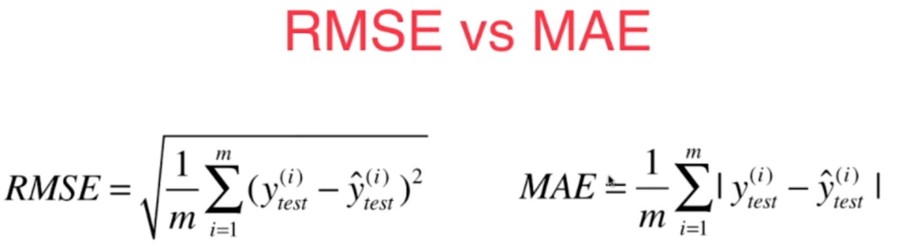
5.衡量线性回归法的指标 MSE,RMS,MAE
当我们跟别人汇报这个衡量标准的时候,这个衡量标准是和m相关的。比如说,你做了一个房产预测的算法,我也做了一个房产预测的算法。然后你说你做的算法,使用这样的标准,最终得到的这个误差的平方的累积的和是1000。我说我的算法得到的是800,那么这样就能说明我的算法更好吗?答案是不能的。因为我们不知道我们两个人在具体进行这个衡量的时候,你的测试数据集有多少,我的测试数据集有多少。那么如果你的测试数据集里有1万个元素,而我的测试数据集里有十个元素,那么在这种情况下,你1万个样本的误差累积起来只有1000可是我十个样本的误差累积起来就达到800了,显然其实是你的算法更好。所以我们可以非常容易的改进一下这个衡量标准,就是给这个式子再除以一个m,相当于让这个衡量标准和我们的测试样本数无关,这个相应的就是一个更为通用的线性回归算法的衡量标准

通常我们对这个标准有一个名词,叫做均方误差。对于这个衡量标准来说其实还有一个小问题,这个问题呢就是量纲上的问题,预测房产,比如说以万元为单位的话,那么这个衡量标准得到的结果其实是万元的平方,这个非常好理解,因为在这里我们y的量纲是万元。那么它平方以后,量纲就变成了万元的平方,把它们都加起来,再除以一个常数,量纲依然是万元的平方。那么这个量纲有的时候可能会为我们带来麻烦,所以一个简单的改进方式
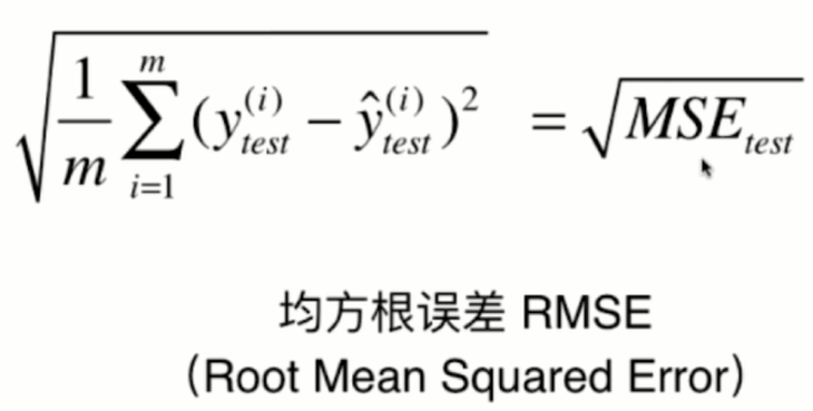
跟这样量纲和我们的y的量纲是一致的。那么这个衡量标准就被称为是均方根误差。其实,RMSE和MSE本质是一样的,虽然这两个数肯定是不同的。他们的区别只在于在具体做报告的时候对这个量纲是否敏感,在有些时候呢,我们使用RSE采用同样的量纲的话,这个误差背后的意义更加明显。
对于线性回归算法还有另外的一个评测标准,这个评测标准非常的直白。
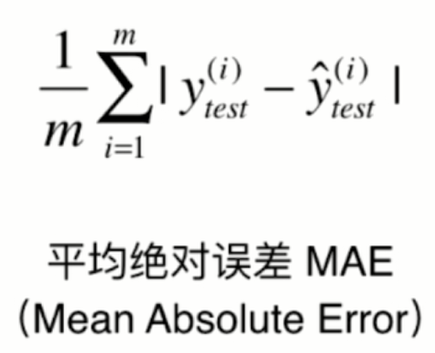
这样的一种衡量方式,它也有一个名字叫做平均绝对误差,英文简称是MAE,这里要注意之前讲线性回归算法在训练的过程中损失函数,或者说是目标函数,没有定成是这个函数是因为那会我们说绝对值它不是一个处处可导的函数,所以它不方便用来求集值。但是这样的一个方法完全可以最终用来评价我们的线性回归算法。我们评价一个算法所使用的标准和我们在训练这个模型的时候,最优化的那个目标函数是可以完全不一致的。
波士顿房产数据
import numpy as np
import matplotlib.pyplot as plt
from sklearn import datasets

boston = datasets.load_boston()
boston.keys()
boston.feature_names
x = boston.data[:,5] # array(['CRIM', 'ZN', 'INDUS', 'CHAS', 'NOX', 'RM', 'AGE', 'DIS', 'RAD',
       #'TAX', 'PTRATIO', 'B', 'LSTAT'], dtype='
x.shape
y = boston.target
y.shape
plt.scatter(x, y)
plt.show()
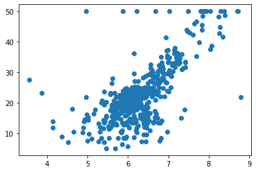
最上一行这50的位置这样分布了一些点,那么这些点呢,看起来俨然是非常奇怪的一些点。事实上,有可能同在真实的世界中获得的数据很多时候也会是这个样子。这些点是我们采集样本拥有的一个上限点,有的时候采集数据的时候,由于各种原因,所以会定一个最大值,那么在我们的这个数据里,所有房产大于50可能是50万美元,这样的房子都被写成了50那么在实际的情况中,有可能是由于你的计量的仪器有一个最大值的限制,或者是你的数据采用问卷的形式,那么用问卷的形式,你设置的问卷中可能有一个最大值在50或者50万美元以上的房子,那么都勾选那同一项,所以就出现了这个最大值的限制,那么对于这些采用最大值的点,显然它有可能不是真实的点。所以在这里我们将这些点给删除掉,那么我们为了再确认一下,我们可以看一下np.max(y)可以确定最大值就是50。现在呢,我们在我们的数据中将所有的外小于50的点抽出来,而外等于等于五十的点呢。就不要了
np.max(y)
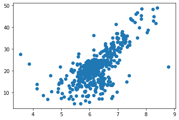
x = x[y < 50.0]
y = y[y < 50.0]
x.shape
y.shape
plt.scatter(x, y)
plt.show()
使用简单线性回归法
from playML.model_selection import train_test_split
x_train, x_test, y_train, y_test = train_test_split(x, y, seed=666)
x_train.shape
y_train.shape
x_test.shape
y_test.shape
from playML.SimpleLinearRegression import SimpleLinearRegression
reg = SimpleLinearRegression()
reg.fit(x_train, y_train)
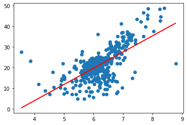
plt.scatter(x_train, y_train)
plt.plot(x_train, reg.predict(x_train), color='r')
plt.show()
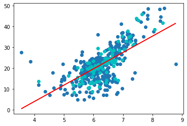
plt.scatter(x_train, y_train)
plt.scatter(x_test, y_test, color="c")
plt.plot(x_train, reg.predict(x_train), color='r')
plt.show()
y_predict = reg.predict(x_test)
MSE
mse_test = np.sum((y_predict - y_test)**2) / len(y_test)
mse_test
输出 24.156602134387438
RMSE
from math import sqrt

rmse_test = sqrt(mse_test)
rmse_test
输出 4.914936635846635
MAE
mae_test = np.sum(np.absolute(y_predict - y_test))/len(y_test)
mae_test
输出 3.5430974409463873
import numpy as np
from math import sqrt


def accuracy_score(y_true, y_predict):
    """计算y_true和y_predict之间的准确率"""
    assert len(y_true) == len(y_predict), \
        "the size of y_true must be equal to the size of y_predict"

    return np.sum(y_true == y_predict) / len(y_true)


def mean_squared_error(y_true, y_predict):
    """计算y_true和y_predict之间的MSE"""
    assert len(y_true) == len(y_predict), \
        "the size of y_true must be equal to the size of y_predict"

    return np.sum((y_true - y_predict)**2) / len(y_true)


def root_mean_squared_error(y_true, y_predict):
    """计算y_true和y_predict之间的RMSE"""

    return sqrt(mean_squared_error(y_true, y_predict))


def mean_absolute_error(y_true, y_predict):
    """计算y_true和y_predict之间的MAE"""

    return np.sum(np.absolute(y_true - y_predict)) / len(y_true)
scikit-learn中的MSE和MAE
from sklearn.metrics import mean_squared_error
from sklearn.metrics import mean_absolute_error

mean_squared_error(y_test, y_predict)
mean_absolute_error(y_test, y_predict)
输出 24.156602134387438 3.5430974409463873
6.最好的衡量线性回归法的指标 R Squared
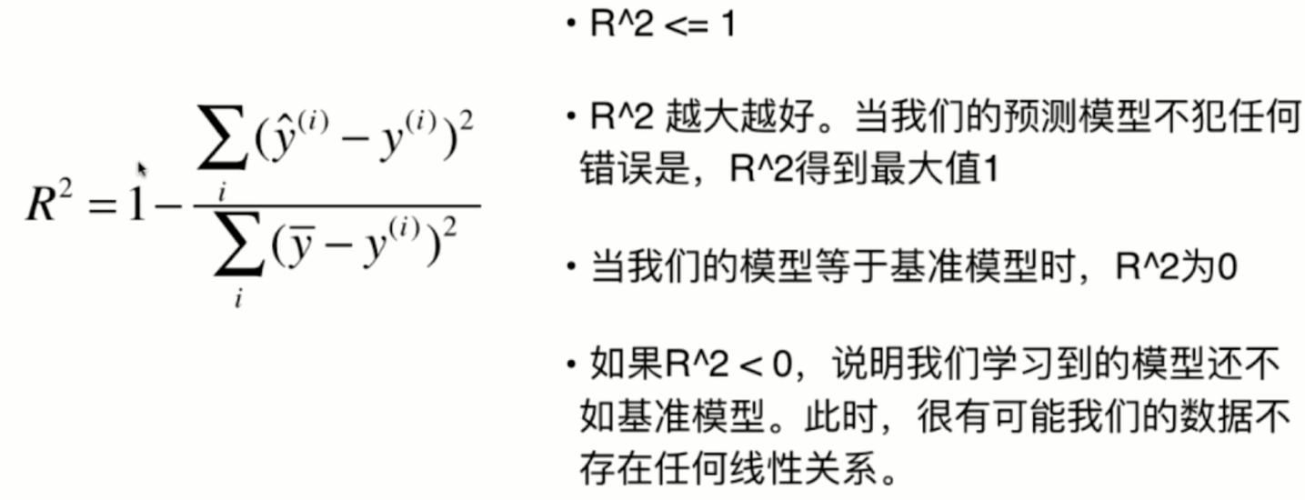
我们讲分类问题的时候,我们评价分类问题的指标非常的简单。就是分类的准确度,对于分类的准确度来说,它的取值是在0-1之间的。如果是1代表它的分类准确度是百分百是最好的,如果是0代表它的分类准确度是0。是最差的,非常的清晰,因为分类的准确度就是在01之间进行取值。即使我们分类的问题不同,我们也可以很容易的来比较他们之间的优劣。
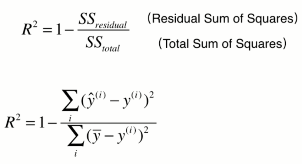
但是,RMSE和MAE是没有这样的性质的,可能我预测的是房产数据,最后得到是5,也就是说的误差是5万元,而预测学生的成绩,可能预测的误差最终的结果是十。也就是预测的差距是十分,那么在这种情况下,请问我们的算法是作用在预测房产中好呢,还是作用在预测学生的成绩中这个问题上好呢。我们是无法判断的,这是因为这个5和10对应的是不同种类的东西。我们无法这样直接比较,这就是我们所使用的RMSE和MAE的局限性。那么,这个问题其实是可以解决的,解决的方法是用一个新的指标,这个指标叫做R Squared。通常我们在中文中也可以叫它是R方,那么R方这个指标,它的计算方法是这样的。
它的意义是什么。

我们可以把这个简单的式子也当做一个模型。只不过这个模型和x是无关的,也就是不管你来什么样的x,我都预测这个结果就是样本的均值。那么它是一个非常朴素的预测结果,对于这样的模型,也有一个相应的名词,叫做baseline model。这个最基本的model,它的错误肯定是比较多的。因为我完全不考虑x直接非常生硬的预测,所有的数据,它都应该等于我的这个样本最终输出结果的均值。而我们的模型预测产生的错误相应的应该是比较少的,因为它充分的考虑了x和y之间的关系。那么基于此,我们就可以这样的来理解这个式子,这个式子描述的就是我们使用baseline 模型来进行预测,会产生非常多的错误。而使用我们自己的模型进行预测,相应的也会产生一些错误,但是同时也会减少一些错误。所以我用1减去我们自己的模型预测产生的错误,在除以我们用baseline model预测产生的错误,最终的结果其实就相当于衡量了我们的模型拟合住的这些数据的地方。相当于是用1减去这个式子就衡量了我们的模型没有产生错误的相应的那个指标。我们就可以得到这些结论。

import numpy as np
import matplotlib.pyplot as plt
from sklearn import datasets

boston = datasets.load_boston()
x = boston.data[:,5] # 只使用房间数量这个特征
y = boston.target

x = x[y < 50.0]
y = y[y < 50.0]

from playML.model_selection import train_test_split

x_train, x_test, y_train, y_test = train_test_split(x, y, seed=666)

from playML.SimpleLinearRegression import SimpleLinearRegression

reg = SimpleLinearRegression()
reg.fit(x_train, y_train)
y_predict = reg.predict(x_test)
封装我们自己的 R Score
import numpy as np
from math import sqrt


def accuracy_score(y_true, y_predict):
    """计算y_true和y_predict之间的准确率"""
    assert len(y_true) == len(y_predict), \
        "the size of y_true must be equal to the size of y_predict"

    return np.sum(y_true == y_predict) / len(y_true)


def mean_squared_error(y_true, y_predict):
    """计算y_true和y_predict之间的MSE"""
    assert len(y_true) == len(y_predict), \
        "the size of y_true must be equal to the size of y_predict"

    return np.sum((y_true - y_predict)**2) / len(y_true)


def root_mean_squared_error(y_true, y_predict):
    """计算y_true和y_predict之间的RMSE"""

    return sqrt(mean_squared_error(y_true, y_predict))


def mean_absolute_error(y_true, y_predict):
    """计算y_true和y_predict之间的MAE"""
    assert len(y_true) == len(y_predict), \
        "the size of y_true must be equal to the size of y_predict"

    return np.sum(np.absolute(y_true - y_predict)) / len(y_true)


def r2_score(y_true, y_predict):
    """计算y_true和y_predict之间的R Square"""

    return 1 - mean_squared_error(y_true, y_predict)/np.var(y_true)
scikit-learn中的 r2_score
from sklearn.metrics import r2_score

r2_score(y_test, y_predict)
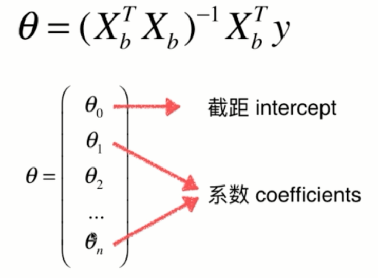
7.多元线性回归和正规方程解
我们之前一直解决的是简单线性回归这样的问题,也就是我们假设我们的样本只有一个特征值。但是在我们的真实世界中,通常一个样本是有很多特征值的,甚至有成千上万个特征值也不奇怪。那么针对这样的样本,我们依然可以使用线性回归的思路来解决这样的问题,那么通常我们就把这样的问题称之为多元线性回归,在这里,我们依然来看这幅图,
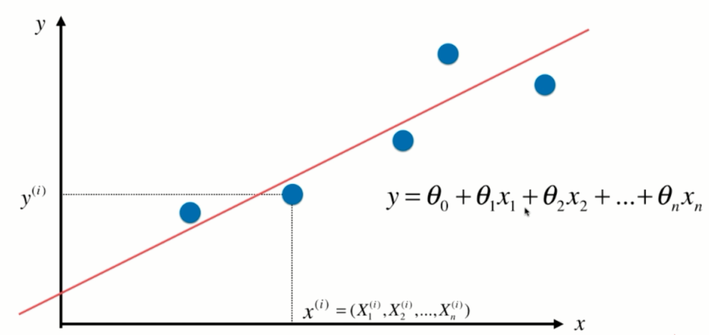
那么在这幅图上,每一个点对应x坐标的一个值,相应的这个值对应y坐标的一个输出的标记,那么当这个xi只是一个数字的时候,对应它其实就是一个简单的线性回归问题。但如果这个xi对应的是一个向量的话,用X表示表示,我们本来有一个大的数据集,每行是一个样本,每一列对应是一个特征。那么,xi对应的就是X,第i行的第1个特征,第i行的第2个特征,依此类推,在这种情况下,其实就是一个多元线性回归问题。我们的数据有多少个特征,有多少个维度。相应的,每一个特征前面都有一个系数,与此同时,这整个一条直线还是有一个截距,在这种情况下,其实所谓的简单线性回归就是我们只需要估计Θ0和Θ1这两个参数的线性回归法。
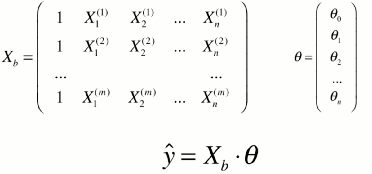
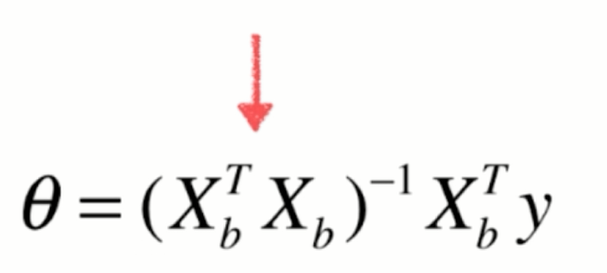
但是在多元线性回归中,相应的,我们就要估计,求出来n+1个参数,那么如果我们可以学习到n+1参数的话。那么对于我们的一个样本,比如说是xi的话,我们就可以这样求出多元线性回归对应的预测值。那么,其实这个形式和我们之前讲的简单线性回归是非常一致的区别,只是我们的特征数从1拓展到了有n个特征,那么其实我们求解这个问题的思路也和简单线性回归方法是一致的。对于简单现象回归来说,我们其实是求一个合适的a和b的值,使这个式子尽可能的小。那么,对于多元线性回归来说,我们依然是使这个式子尽可能的小,因为这个式子表达的意思就是我们预测的结果和真实的结果,他们之间的差的平方的和。我们要让这个式子尽可能的小。


8.实现多元线性回归
广义上的线性回归模型,也就是支持多元线性回归这样的方式
import numpy as np
from .metrics import r2_score

class LinearRegression:

    def __init__(self):
        """初始化Linear Regression模型"""
        self.coef_ = None
        self.intercept_ = None
        self._theta = None

    def fit_normal(self, X_train, y_train):
        """根据训练数据集X_train, y_train训练Linear Regression模型"""
        assert X_train.shape[0] == y_train.shape[0], \
            "the size of X_train must be equal to the size of y_train"

        X_b = np.hstack([np.ones((len(X_train), 1)), X_train])
        self._theta = np.linalg.inv(X_b.T.dot(X_b)).dot(X_b.T).dot(y_train)

        self.intercept_ = self._theta[0]
        self.coef_ = self._theta[1:]

        return self

    def predict(self, X_predict):
        """给定待预测数据集X_predict,返回表示X_predict的结果向量"""
        assert self.intercept_ is not None and self.coef_ is not None, \
            "must fit before predict!"
        assert X_predict.shape[1] == len(self.coef_), \
            "the feature number of X_predict must be equal to X_train"

        X_b = np.hstack([np.ones((len(X_predict), 1)), X_predict])
        return X_b.dot(self._theta)

    def score(self, X_test, y_test):
        """根据测试数据集 X_test 和 y_test 确定当前模型的准确度"""

        y_predict = self.predict(X_test)
        return r2_score(y_test, y_predict)

    def __repr__(self):
        return "LinearRegression()"
实现我们自己的 Linear Regression
import numpy as np
import matplotlib.pyplot as plt
from sklearn import datasets

boston = datasets.load_boston()

X = boston.data
y = boston.target

X = X[y < 50.0]
y = y[y < 50.0]

from playML.model_selection import train_test_split

X_train, X_test, y_train, y_test = train_test_split(X, y, seed=666)

from playML.LinearRegression import LinearRegression

reg = LinearRegression()
reg.fit_normal(X_train, y_train)
reg.coef_
array([-1.20354261e-01, 3.64423279e-02, -3.61493155e-02, 5.12978140e-02, -1.15775825e+01, 3.42740062e+00, -2.32311760e-02, -1.19487594e+00, 2.60101728e-01, -1.40219119e-02, -8.35430488e-01, 7.80472852e-03, -3.80923751e-01])
reg.intercept_
34.117399723201785
reg.score(X_test, y_test)
0.8129794056212823
scikit-learn中的回归问题
from sklearn.linear_model import LinearRegression

lin_reg = LinearRegression()
lin_reg.fit(X_train, y_train)
kNN Regressor
from sklearn.preprocessing import StandardScaler

standardScaler = StandardScaler()
standardScaler.fit(X_train, y_train)
X_train_standard = standardScaler.transform(X_train)
X_test_standard = standardScaler.transform(X_test)

from sklearn.neighbors import KNeighborsRegressor

knn_reg = KNeighborsRegressor()
knn_reg.fit(X_train_standard, y_train)
knn_reg.score(X_test_standard, y_test)

from sklearn.model_selection import GridSearchCV

param_grid = [
    {
        "weights": ["uniform"],
        "n_neighbors": [i for i in range(1, 11)]
    },
    {
        "weights": ["distance"],
        "n_neighbors": [i for i in range(1, 11)],
        "p": [i for i in range(1,6)]
    }
]

knn_reg = KNeighborsRegressor()
grid_search = GridSearchCV(knn_reg, param_grid, n_jobs=-1, verbose=1)
grid_search.fit(X_train_standard, y_train)