【无标题】pytorch构建利用迁移学习MNIST数据集的加法器实验
文章目录
- 前言
- 一、pytorch构建利用迁移学习MNIST数据集的加法器实验要求
- 二、各个python文件
-
- 1.main.py
- 2.network4.py
- 3.data_loader.py
- 三、实验过程
-
- 总结
前言
迁移学习可以将在一个领域训练的机器学习模型应用到另一个领域,在某种程度上提高了训练模型的利用率,解决了数据缺失的问题,并赋予了智能模型“举一反三”的能力。本实验以之前训练的MNIST手写数字识别模型为基础,实现一个手写数字加法机。
一、pytorch构建利用迁移学习MNIST数据集的加法器实验要求
- 输入两张手写数字图像,输出这两个数字的和。
- 利用综合实验三搭建的神经网络。
- 项目文件夹里面有一个文件夹以及三个文件,文件夹名为data,存放MNIST数据集,三个文件为: main.py、network4.py、 data_loader.py。main为主文件,;network4.py存放神经网络类定义及相关函数;data_loader.py存放负责读入数据的相关方法。
二、各个python文件
1.main.py
代码如下:
import network4
import data_loader
import torch.optim as optim
import torch.nn as nn
import matplotlib.pyplot as plt
from torch.autograd import Variable
import pylab
import torch
import warnings


if __name__=="__main__":
    warnings.filterwarnings("ignore")
    net0 = network4.Transfer()  # 没有迁移的网络
    net1 =network4.Transfer()   # 迁移没固定的网络
    net2 =network4.Transfer()   # 迁移固定的网络
    original_net = network4.ConvNet() #之前的手写数字识别的卷积神经网络
    state_dict = torch.load('model_new902')  # 加载之前的手写数字识别的卷积神经网络保存下来的模型model_new902
    original_net.load_state_dict(state_dict)
    """
    =======================================     ====================================================
    # cycle_training(net,num_epochs=20)         让新的加法机全部重新训练

    # cycle_training_to_transfer_pretrained     将旧的手写数字识别的卷积神经网络权重迁移过来,作为新的加法机网络来
    (net,original_net,num_epochs=20):           训练

    # cycle_training_to_transfer_fixed          将旧的手写数字识别的卷积层的权重全部迁移到了加法机的两个卷积部件中,
    (net,original_net,num_epochs=20)            但之后保持它们的权重不变,只允许后面的全链接层的权重可训练
    =======================================     ====================================================
    """

    result0= network4.cycle_training(net0,num_epochs=20)
    result1=network4.cycle_training_to_transfer_pretrained(net1,original_net,num_epochs=20)
    result2=network4.cycle_training_to_transfer_fixed(net2,original_net,num_epochs=20)
    network4.show_different_network_training_result(result0[0],result1[0],result2[0]) #展示不同方式训练的加法器网络的效果
    # result_save={'no_transfer':result0,'transfer_pretrained':result1,'transfer_fixed':result2} #将结果转成字典
    # network4.save_results_to_file("pre_data/result903.json",result_save)  # 结果保存到文件
2.network4.py
代码如下:
import torch
import torch.nn as nn
import torch.nn.functional as F
import torch.optim as optim
from data_loader import *
import copy
import matplotlib.pyplot as plt
import json
import os

use_save = False #是否将所有运行结果保存下来
save_txt_path='pre_data/result.txt' # 输出结果保存成txt的文件路径
save_figure_path='pre_data/' # 输出图片保存的文件路径
if use_save:
    path_dirname = os.path.dirname(__file__)
    base_path = os.path.join(path_dirname, save_figure_path.replace('/',''))
    if not os.path.exists(base_path):
        os.makedirs(base_path)
use_cuda = torch.cuda.is_available() #定义一个布尔型变量,标志当前的GPU是否可用
# 如果当前GPU可用,则将优先在GPU上进行张量计算
dtype = torch.cuda.FloatTensor if use_cuda else torch.FloatTensor
itype = torch.cuda.LongTensor if use_cuda else torch.LongTensor
# 定义卷积神经网络:6和16为人为指定的两个卷积层
depth = [6, 16]
image_size = 28  #图像的总尺寸28*28
num_classes = 10  #标签的种类数
num_epochs = 20  #训练的总循环周期
batch_size = 64  #批处理的尺寸大小

class ConvNet(nn.Module):
    def __init__(self):
        super(ConvNet, self).__init__()
        self.conv1 = nn.Conv2d(1, depth[0], 5, padding=2)  # 定义一个卷积层,输入通道为1,输出通道为6,窗口大小为5,padding为2
        self.pool = nn.MaxPool2d(2, 2)  # 定义一个池化层,一个窗口为2x2的池化运箅
        # 第二层卷积,输入通道为depth[o],输出通道为depth[1],窗口为 5,padding 为2
        self.conv2 = nn.Conv2d(depth[0], depth[1], 5, padding=2)  # 输出通道为depth[1],窗口为5,padding为2
        # 一个线性连接层,输入尺寸为最后一层立方体的线性平铺,输出层 512个节点
        self.fc1 = nn.Linear(image_size // 4 * image_size // 4 * depth[1], 512)
        # 最后一层线性分类单元,输入为 512,输出为要做分类的类别数
        self.fc2 = nn.Linear(512, num_classes)

    def forward(self, x):  # 该函数完成神经网络真正的前向运算,在这里把各个组件进行实际的拼装
        x = self.conv1(x)  # 第一层卷积
        x = F.relu(x)  # 激活函数用ReLU,防止过拟合
        x = self.pool(x)  # 第二层池化,将图片变小
        x = self.conv2(x)  # 第三层又是卷积,窗口为5,输入输出通道分列为depth[o]=4,depth[1]=8
        x = F.relu(x)  # 非线性函数
        x = self.pool(x)  # 第四层池化,将图片缩小到原来的 1/4
        # 将立体的特征图 tensor 压成一个一维的向量
        # view 函数可以将一个tensor 按指定的方式重新排布
        x = x.view(-1, image_size // 4 * image_size // 4 * depth[1])
        x = F.relu(self.fc1(x))  # 第五层为全连接,ReLU激活函数
        # 以默认0.5的概率对这一层进行dropout操作,防止过拟合
        x = F.dropout(x, training=self.training)
        x = self.fc2(x)  # 全连接
        # 输出层为 log_Softmax,即概率对数值 log(p(×))。采用log_softmax可以使后面的交叉熵计算更快
        x = F.log_softmax(x, dim=1)
        return x


def rightness(predictions, labels):
    """计算预测错误率的函数,其中predictions是模型给出的一组预测结果,batch_size行10列的矩阵,labels是数据之中的正确答案"""
    pred = torch.max(predictions.data, 1)[1]  # 对于任意一行(一个样本)的输出值的第1个维度,求最大,得到每一行的最大元素的下标
    rights = pred.eq(labels.data.view_as(pred)).sum()  # 将下标与labels中包含的类别进行比较,并累计得到比较正确的数量
    return rights, len(labels)  # 返回正确的数量和这一次一共比较了多少元素


def show_testset_total_accuracy(model:str):
    """
    展示模型在原始的网络上的准确率
    Show the accuracy of the model on the original network
    """
    original_net =ConvNet()
    state_dict=torch.load(model)
    original_net.load_state_dict(state_dict)
    print(original_net) #将网络打印出来观看
    # 在测试集上分批运行,并计算总的正确率
    original_net.eval()  # 标志模型当前为运行阶段
    test_loss = 0
    correct = 0
    vals = []

    # 对测试数据集进行循环
    for data, target in test_loader1:
        with torch.no_grad():
            data = data.clone().detach()
        target = target.clone().detach()
        output = original_net(data)  # 将特征数据喂入网络,得到分类的输出
        val = rightness(output, target)  # 获得正确样本数以及总样本数
        vals.append(val)  # 记录结果

    # 计算模型在测试集上的准确率
    rights = (sum([tup[0] for tup in vals]), sum([tup[1] for tup in vals]))
    right_rate = 1.0 * rights[0].numpy() / rights[1]
    print("{}模型在测试集上的准确率:{:.2f}%".format(model,100.0*right_rate))

def read_a_picture(index):
    """
    随便从测试集中读入一张图片,并绘制出来
    Read a picture randomly from the test set and draw it
    """

    idx = index
    muteimg = test_dataset[idx][0].numpy()
    plt.imshow(muteimg[0, ...])
    label=test_dataset[idx][1]
    print('标签是:', label)
    plt.title(str(label))
    plt.show()

def read_two_picture(index1,index2):
    """
    随便从测试集中读入两张图片,并绘制出来
    Read two picture randomly from the test set and draw them

    """

    idx1 = index1
    idx2 = index2
    muteimg1 = test_dataset[idx1][0].numpy()
    muteimg2 = test_dataset[idx2][0].numpy()
    label1 = test_dataset[idx1][1]
    label2 = test_dataset[idx2][1]
    fig, axes = plt.subplots(1,2)  # 创建图实例
    axes[0].imshow(muteimg1[0, ...])
    axes[0].set_title(str(label1))
    axes[1].imshow(muteimg2[0, ...])
    axes[1].set_title(str(label2))
    print('两张图片标签分别是:', label1,label2)
    plt.show()  # 图形可视化

def add_two_pictures_using_the_network(transfer_net,index1=1,index2=2):
    """
    Read two pictures randomly from the test set and add them on the network
    随便从测试集中读入两张图片,并用网络做加法

    """
    with torch.no_grad():
        img1, label1 = test_dataset[index1]
        img2, label2 = test_dataset[index2]
        label_total=label1+label2
        img1=torch.tensor(img1).unsqueeze(dim=0)
        img2 = torch.tensor(img2).unsqueeze(dim=0)
        # print(img1.size(),img2.size())
        outputs = transfer_net(img1,img2)   # .clone().detach().requires_grad_(True)
        _, predicted = torch.max(outputs.data, 1)
        predicted_label_total=predicted.squeeze().numpy()
        print("真实标签A: {} ,真实标签B: {} ,  两个标签的真实和: {}\t 网络预测标签和: {}".format(
            label1,label2,label_total,predicted_label_total))
        read_two_picture(index1,index2)


# =========== 数字加法机 ============
# 数字加法机:输入两张图像,输出这两个手写数字的加法。
class Transfer(nn.Module):
    def __init__(self):
        super(Transfer, self).__init__()
        # 两个并行的卷积通道,第一个通道:
        self.net1_conv1 = nn.Conv2d(1,depth[0] , 5, padding=2)  # 一个输入通道,6个输出通道(6个卷积核),窗口为5,填充2
        self.net_pool = nn.MaxPool2d(2, 2)  # 2*2 池化
        self.net1_conv2 = nn.Conv2d(depth[0], depth[1], 5, padding=2)  # 输入通道4,输出通道16(16个卷积核),窗口5,填充2

        # 第二个通道,注意pooling操作不需要重复定义
        self.net2_conv1 = nn.Conv2d(1, depth[0], 5, padding=2)  # 一个输入通道,6个输出通道(6个卷积核),窗口为5,填充2
        self.net2_conv2 = nn.Conv2d(depth[0], depth[1], 5, padding=2)  # 输入通道4,输出通道16(16个卷积核),窗口5,填充2

        # 全链接层
        self.fc1 = nn.Linear(2 * image_size // 4 * image_size // 4 * depth[1], 1024)  # 输入为处理后的特征图压平,输出1024个单元
        self.fc2 = nn.Linear(1024, 256)  # 输入1024个单元,输出256个单元
        self.fc3 = nn.Linear(256, 64)  # 输入256个单元,输出64个单元
        self.fc4 = nn.Linear(64,19)  # 输入64个单元,输出为19

    def forward(self, x, y, training=True):
        # 网络的前馈过程。输入两张手写图像x和y,输出一个数字表示两个数字的和
        # x,y都是batch_size*image_size*image_size形状的三阶张量
        # 输出为batch_size长的列向量

        # 首先,第一张图像进入第一个通道
        x = F.relu(self.net1_conv1(x))  # 第一层卷积
        x = self.net_pool(x)  # 第一层池化
        x = F.relu(self.net1_conv2(x))  # 第二层卷积
        x = self.net_pool(x)  # 第二层池化
        x = x.view(-1, image_size // 4 * image_size // 4 * depth[1])  # 将特征图张量压平

        y = F.relu(self.net2_conv1(y))  # 第一层卷积
        y = self.net_pool(y)  # 第一层池化
        y = F.relu(self.net2_conv2(y))  # 第二层卷积
        y = self.net_pool(y)  # 第二层池化
        y = y.view(-1, image_size // 4 * image_size // 4 * depth[1])  # 将特征图张量压平

        # 将两个卷积过来的铺平向量拼接在一起,形成一个大向量
        z = torch.cat((x, y), 1)  # cat函数为拼接向量操作,1表示拼接的维度为第1个维度(0维度对应了batch)
        z = self.fc1(z)  # 第一层全链接
        z = F.relu(z)  # 对于深层网络来说,激活函数用relu效果会比较好
        z = F.dropout(z, training=self.training)  # 以默认为0.5的概率对这一层进行dropout操作
        z = self.fc2(z)  # 第二层全链接
        z = F.relu(z)
        z = self.fc3(z)  # 第三层全链接
        z = F.relu(z)
        z = self.fc4(z)  # 第四层全链接
        return z

    def set_filter_values(self, net):
        # 本函数为迁移网络所用,即将迁移过来的网络的权重值拷贝到本网络中
        # 本函数对应的迁移为预训练式
        # 输入参数net为从硬盘加载的网络作为迁移源

        # 逐个儿为网络的两个卷积模块的权重和偏置进行赋值
        # 注意在赋值的时候需要用deepcopy而不能直接等于,或者copy。
        # 这是因为这种拷贝是将张量中的数值全部拷贝到了目标中,而不是拷贝地址
        # 如果不用deepcopy,由于我们将同一组参数(net.conv1.weight.data,bias)
        #  赋予了两组参数(net1_conv1.weight.data,net2_conv1.weight.data)
        # 所以它们会共享源net.conv1.weight.data中的地址,这样对于net1_conv1.weight.data
        # 的训练也自然会被用到了net2_conv1.weight.data中,但其实我们希望它们是两个不同的参数。
        self.net1_conv1.weight.data = copy.deepcopy(net.conv1.weight.data)
        self.net1_conv1.bias.data = copy.deepcopy(net.conv1.bias.data)
        self.net1_conv2.weight.data = copy.deepcopy(net.conv2.weight.data)
        self.net1_conv2.bias.data = copy.deepcopy(net.conv2.bias.data)
        self.net2_conv1.weight.data = copy.deepcopy(net.conv1.weight.data)
        self.net2_conv1.bias.data = copy.deepcopy(net.conv1.bias.data)
        self.net2_conv2.weight.data = copy.deepcopy(net.conv2.weight.data)
        self.net2_conv2.bias.data = copy.deepcopy(net.conv2.bias.data)

        # 将变量加载到GPU上
        self.net1_conv1 = self.net1_conv1.cuda() if use_cuda else self.net1_conv1
        self.net1_conv2 = self.net1_conv2.cuda() if use_cuda else self.net1_conv2

        self.net2_conv1 = self.net2_conv1.cuda() if use_cuda else self.net2_conv1
        self.net2_conv2 = self.net2_conv2.cuda() if use_cuda else self.net2_conv2

    def set_filter_values_nograd(self, net):
        # 本函数为迁移网络所用,即将迁移过来的网络的权重值拷贝到本网络中
        # 本函数对应的迁移为固定权重式
        # 调用set_filter_values为全部卷积核进行赋值
        self.set_filter_values(net)

        # 为了让我们的网络不被训练调整权值,我们需要设定每一个变量的requires_grad为False
        # 即不需要计算梯度值
        self.net1_conv1.weight.requires_grad = False
        self.net1_conv1.bias.requires_grad = False
        self.net1_conv2.weight.requires_grad = False
        self.net1_conv2.bias.requires_grad = False

        self.net2_conv1.weight.requires_grad = False
        self.net2_conv1.bias.requires_grad = False
        self.net2_conv2.weight.requires_grad = False
        self.net2_conv2.bias.requires_grad = False

def rightness_add(y, target):
    # 计算分类准确度的函数,y为模型预测的标签,target为数据的标签
    # 输入的y为一个矩阵,行对应了batch中的不同数据记录,列对应了不同的分类选择,数值对应了概率
    # 函数输出分别为预测与数据标签相等的个数,本次判断的所有数据个数
    preds = y.data.max(dim=1, keepdim=True)[1]
    return (preds.eq(target.data.view_as(preds)).cpu().sum(), len(target))

def cycle_training(net,num_epochs=20):
    fraction = 1
    if use_cuda:
        net = net.cuda()

    criterion = nn.CrossEntropyLoss()
    optimizer = optim.SGD(net.parameters(), lr=0.01, momentum=0.9)
    records = []  # 记录准确率等数值的容器
    # 开始训练网络
    for epoch in range(num_epochs):
        train_rights = []  # 记录训练数据集准确率的容器
        losses = []
        for idx, data in enumerate(zip(train_loader1, train_loader2)):
            if idx >= (len(train_loader1) // fraction):
                break
            ((x1, y1), (x2, y2)) = data
            if use_cuda:
                x1, y1, x2, y2 = x1.cuda(), y1.cuda(), x2.cuda(), y2.cuda()
            net.train()
            optimizer.zero_grad()
            outputs = net(x1.clone().detach().requires_grad_(True), x2.clone().detach().requires_grad_(True))
            labels = y1 + y2
            loss = criterion(outputs, labels.type(torch.long))
            loss.backward()
            optimizer.step()
            loss = loss.cpu() if use_cuda else loss
            losses.append(loss.data.numpy())
            right = rightness_add(outputs.data, labels)  # 计算准确率所需数值,返回数值为(正确样例数,总样本数)
            train_rights.append(right)  # 将计算结果装到列表容器train_rights中
            if (idx + 1) % n_batch == 0:
                val_rights = []  # 记录校验数据集准确率的容器
                val_losses = []
                net.eval()
                for val_data in zip(val_loader1, val_loader2):
                    ((x1, y1), (x2, y2)) = val_data
                    if use_cuda:
                        x1, y1, x2, y2 = x1.cuda(), y1.cuda(), x2.cuda(), y2.cuda()
                    outputs = net(x1.clone().detach().requires_grad_(True), x2.clone().detach().requires_grad_(True))
                    labels = y1 + y2
                    loss = criterion(outputs, labels.type(torch.long))
                    loss = loss.cpu() if use_cuda else loss
                    val_losses.append(loss.data.numpy())

                    right = rightness_add(outputs.data, labels)
                    val_rights.append(right)
                epoch_index = epoch + (idx + 1) / len(train_loader1)
                train_right_ratio = 1.0 * np.sum([i[0].cpu().numpy() for i in train_rights]) / np.sum(
                    [i[1] for i in train_rights])
                val_right_ratio = 1.0 * np.sum([i[0].cpu().numpy() for i in val_rights]) / np.sum(
                    [i[1] for i in val_rights])
                if use_save:
                    with open(save_txt_path,'a') as fw:
                        fw.write('训练周期: {} [{}/{} ({:.0f}%)]\t 训练误差:{:.2f}  校验误差:{:.2f}  训练准确率:{:.2f}%  验证准确率:{:.2f}%\n'.format(
                    epoch, idx * batch_size, training_set_size, 100. * (idx + 1) / len(train_loader1),
                    np.mean(losses), np.mean(val_losses), 100. * train_right_ratio, 100. * val_right_ratio))

                print('训练周期: {} [{}/{} ({:.0f}%)]\t 训练误差:{:.2f}  校验误差:{:.2f}  训练准确率:{:.2f}%  验证准确率:{:.2f}%'.format(
                    epoch, idx * batch_size, training_set_size, 100. * (idx + 1) / len(train_loader1),
                    np.mean(losses), np.mean(val_losses), 100. * train_right_ratio, 100. * val_right_ratio))
                records.append([epoch_index, np.mean(losses), np.mean(val_losses), train_right_ratio, val_right_ratio])
                train_rights = []
                val_rights = []
    test_rights = []
    net.eval()
    for test_data in zip(test_loader1, test_loader2):
        ((x1, y1), (x2, y2)) = test_data
        if use_cuda:
            x1, y1, x2, y2 = x1.cuda(), y1.cuda(), x2.cuda(), y2.cuda()
        outputs = net(x1.clone().detach().requires_grad_(True), x2.clone().detach().requires_grad_(True))
        labels = y1 + y2
        # loss = criterion(outputs, labels.type(torch.long))
        right = rightness_add(outputs.data, labels)
        test_rights.append(right)
    test_right_ratio = 1.0 * np.sum([i[0].cpu().numpy() for i in test_rights]) / np.sum([i[1] for i in test_rights])
    print("最终测试集准确率:{:.2f}%".format(100. * test_right_ratio))
    if use_save:
        with open(save_txt_path, 'a') as fw:
            fw.write("最终测试集准确率:{:.2f}%\n".format(100.*test_right_ratio))
    results = [records, test_right_ratio]
    fig, ax = plt.subplots()
    ax.plot([j[0] for j in records], [i[3] for i in records], c='r', label='Train')
    ax.plot([j[0] for j in records], [i[4] for i in records], c='b', label='Validation')
    ax.legend()
    ax.set_ylabel('accuracy')
    ax.set_xlabel('epoch')
    ax.set_title('no transfer Accuracy')
    if use_save:
        plt.savefig(str(save_figure_path+'no_transfer_Accuracy.png'))
    else:
        plt.show()
    return results


def cycle_training_to_transfer_pretrained(net,original_net,num_epochs=20):
    # 为了比较不同数据量对迁移学习的影响,我们设定了一个加载数据的比例fraction
    # 即我们只加载原训练数据集的1/fraction来训练网络
    fraction = 1
    # 为新网络赋予权重数值,注意我们只将卷积部分的网络进行迁移,而没有迁移全链接层
    net.set_filter_values(original_net)

    if use_cuda:
        net = net.cuda()

    criterion = nn.CrossEntropyLoss()

    # 将需要训练的参数加载到优化器中
    new_parameters = []
    for para in net.parameters():
        if para.requires_grad:  # 我们只将可以调整权重的变量加到了集合new_parameters
            new_parameters.append(para)

    # 将new_parameters加载到了优化器中
    optimizer = optim.SGD(new_parameters, lr=0.01, momentum=0.9)
    records = [] # 记录准确率等数值的容器
    # 开始训练网络
    for epoch in range(num_epochs):
        train_rights = []  # 记录训练数据集准确率的容器
        losses = []
        for idx, data in enumerate(zip(train_loader1, train_loader2)):
            if idx >= (len(train_loader1) // fraction):
                break
            ((x1, y1), (x2, y2)) = data
            if use_cuda:
                x1, y1, x2, y2 = x1.cuda(), y1.cuda(), x2.cuda(), y2.cuda()
            net.train()
            optimizer.zero_grad()
            outputs = net(x1.clone().detach().requires_grad_(True), x2.clone().detach().requires_grad_(True))
            labels = y1 + y2
            loss = criterion(outputs, labels.type(torch.long))
            loss.backward()
            optimizer.step()
            loss = loss.cpu() if use_cuda else loss
            losses.append(loss.data.numpy())
            right = rightness_add(outputs.data, labels)  # 计算准确率所需数值,返回数值为(正确样例数,总样本数)
            train_rights.append(right)  # 将计算结果装到列表容器train_rights中
            if (idx+1) % n_batch == 0:
                val_rights = []  # 记录校验数据集准确率的容器
                val_losses = []
                net.eval()
                for val_data in zip(val_loader1, val_loader2):
                    ((x1, y1), (x2, y2)) = val_data
                    if use_cuda:
                        x1, y1, x2, y2 = x1.cuda(), y1.cuda(), x2.cuda(), y2.cuda()
                    outputs = net(x1.clone().detach().requires_grad_(True), x2.clone().detach().requires_grad_(True))
                    labels = y1 + y2
                    loss = criterion(outputs, labels.type(torch.long))
                    loss = loss.cpu() if use_cuda else loss
                    val_losses.append(loss.data.numpy())

                    right = rightness_add(outputs.data, labels)
                    val_rights.append(right)
                epoch_index=epoch+(idx+1)/len(train_loader1)
                train_right_ratio=1.0 * np.sum([i[0].cpu().numpy() for i in train_rights]) / np.sum([i[1] for i in train_rights])
                val_right_ratio = 1.0 * np.sum([i[0].cpu().numpy() for i in val_rights]) / np.sum([i[1] for i in val_rights])

                if use_save:
                    with open(save_txt_path, 'a') as fw:
                        fw.write(
                            '训练周期: {} [{}/{} ({:.0f}%)]\t 训练误差:{:.2f}  校验误差:{:.2f}  训练准确率:{:.2f}%  验证准确率:{:.2f}%\n'.format(
                                epoch, idx * batch_size, training_set_size, 100. * (idx + 1) / len(train_loader1),
                                np.mean(losses), np.mean(val_losses), 100. * train_right_ratio, 100. * val_right_ratio))

                print('训练周期: {} [{}/{} ({:.0f}%)]\t 训练误差:{:.2f}  校验误差:{:.2f}  训练准确率:{:.2f}%  验证准确率:{:.2f}%'.format(
                    epoch, idx*batch_size, training_set_size,100. * (idx+1) / len(train_loader1),
                    np.mean(losses), np.mean(val_losses), 100.*train_right_ratio,100.*val_right_ratio))
                records.append([epoch_index,np.mean(losses), np.mean(val_losses), train_right_ratio,val_right_ratio])
                train_rights = []
                val_rights = []
    test_rights = []
    net.eval()
    for test_data in zip(test_loader1, test_loader2):
        ((x1, y1), (x2, y2)) = test_data
        if use_cuda:
            x1, y1, x2, y2 = x1.cuda(), y1.cuda(), x2.cuda(), y2.cuda()
        outputs = net(x1.clone().detach().requires_grad_(True), x2.clone().detach().requires_grad_(True))
        labels = y1 + y2
        # loss = criterion(outputs, labels.type(torch.long))
        right = rightness_add(outputs.data, labels)
        test_rights.append(right)
    test_right_ratio = 1.0 * np.sum([i[0].cpu().numpy() for i in test_rights]) / np.sum([i[1] for i in test_rights])
    print("最终测试集准确率:{:.2f}%".format(100.*test_right_ratio))
    if use_save:
        with open(save_txt_path, 'a') as fw:
            fw.write("最终测试集准确率:{:.2f}%\n".format(100.*test_right_ratio))

    results=[records, test_right_ratio]
    fig,ax=plt.subplots()
    ax.plot([j[0] for j in records],[i[3] for i in records],c='r',label='Train')
    ax.plot([j[0] for j in records],[i[4] for i in records],c='b',label='Validation')
    ax.legend()
    ax.set_ylabel('accuracy')
    ax.set_xlabel('epoch')
    ax.set_title('Transfer pretrained Accuracy')

    if use_save:
        plt.savefig(str(save_figure_path + 'Transfer_pretrained_Accuracy.png'))
    else:
        plt.show()

    return results


def cycle_training_to_transfer_fixed(net,original_net,num_epochs=20):
    # 为了比较不同数据量对迁移学习的影响,我们设定了一个加载数据的比例fraction
    # 即我们只加载原训练数据集的1/fraction来训练网络
    fraction = 1
    # 在这个试验中,我们首先将识别器的卷积层的权重全部迁移到了加法机的两个卷积部件中,
    # 但保持它们的权重不变,只允许后面的全链接层的权重可训练

    # 迁移网络,并设置卷积部件的权重和偏置都不计算梯度
    net.set_filter_values_nograd(original_net)
    if use_cuda:
        net = net.cuda()
    criterion = nn.CrossEntropyLoss()

    # 只将可更新的权重值加载到了优化器中
    new_parameters = []
    for para in net.parameters():
        if para.requires_grad:
            new_parameters.append(para)
    optimizer = optim.SGD(new_parameters, lr=0.01, momentum=0.9)
    # 训练整个网络
    records = []
    for epoch in range(num_epochs):
        losses = []
        train_rights = []  # 记录训练数据集准确率的容器
        for idx, data in enumerate(zip(train_loader1, train_loader2)):
            if idx >= (len(train_loader1) // fraction):
                break
            ((x1, y1), (x2, y2)) = data
            if use_cuda:
                x1, y1, x2, y2 = x1.cuda(), y1.cuda(), x2.cuda(), y2.cuda()
            net.train()
            optimizer.zero_grad()
            outputs = net(x1.clone().detach().requires_grad_(True), x2.clone().detach().requires_grad_(True))
            labels = y1 + y2
            loss = criterion(outputs, labels.type(torch.long))
            loss.backward()

            optimizer.step()
            loss = loss.cpu() if use_cuda else loss
            losses.append(loss.data.numpy())
            right = rightness_add(outputs.data, labels)  # 计算准确率所需数值,返回数值为(正确样例数,总样本数)
            train_rights.append(right)  # 将计算结果装到列表容器train_rights中
            if (idx+1) % n_batch == 0:
                val_rights = []  # 记录校验数据集准确率的容器
                val_losses = []
                net.eval()
                for val_data in zip(val_loader1, val_loader2):
                    ((x1, y1), (x2, y2)) = val_data
                    if use_cuda:
                        x1, y1, x2, y2 = x1.cuda(), y1.cuda(), x2.cuda(), y2.cuda()
                    outputs = net(x1.clone().detach().requires_grad_(True), x2.clone().detach().requires_grad_(True))
                    labels = y1 + y2
                    loss = criterion(outputs, labels.type(torch.long))
                    loss = loss.cpu() if use_cuda else loss
                    val_losses.append(loss.data.numpy())
                    right = rightness(outputs.data, labels)
                    val_rights.append(right)
                epoch_index = epoch + (idx+1) / len(train_loader1)
                train_right_ratio = 1.0 * np.sum([i[0].cpu().numpy() for i in train_rights]) / np.sum(
                    [i[1] for i in train_rights])
                val_right_ratio = 1.0 * np.sum([i[0].cpu().numpy() for i in val_rights]) / np.sum(
                    [i[1] for i in val_rights])
                if use_save:
                    with open(save_txt_path, 'a') as fw:
                        fw.write(
                            '训练周期: {} [{}/{} ({:.0f}%)]\t 训练误差:{:.2f}  校验误差:{:.2f}  训练准确率:{:.2f}%  验证准确率:{:.2f}%\n'.format(
                                epoch, idx * batch_size, training_set_size, 100. * (idx + 1) / len(train_loader1),
                                np.mean(losses), np.mean(val_losses), 100. * train_right_ratio, 100. * val_right_ratio))

                print('训练周期: {} [{}/{} ({:.0f}%)]\t 训练误差:{:.2f}  校验误差:{:.2f}  训练准确率:{:.2f}%  验证准确率:{:.2f}%'.format(
                    epoch, idx * batch_size, training_set_size, 100. * (idx+1) / len(train_loader1),
                    np.mean(losses), np.mean(val_losses), 100. * train_right_ratio, 100. * val_right_ratio))
                records.append([epoch_index,np.mean(losses), np.mean(val_losses), train_right_ratio,val_right_ratio])
                train_rights=[]
                val_rights=[]
    test_rights = []
    net.eval()
    for test_data in zip(test_loader1, test_loader2):
        ((x1, y1), (x2, y2)) = test_data
        if use_cuda:
            x1, y1, x2, y2 = x1.cuda(), y1.cuda(), x2.cuda(), y2.cuda()
        outputs = net(x1.clone().detach().requires_grad_(True), x2.clone().detach().requires_grad_(True))
        labels = y1 + y2
        loss = criterion(outputs, labels.type(torch.long))
        right = rightness(outputs.data, labels)
        test_rights.append(right)
    test_right_ratio = 1.0 * np.sum([i[0].cpu().numpy() for i in test_rights]) / np.sum([i[1] for i in test_rights])
    print("最终测试集准确率:{:.2f}%".format(100. * test_right_ratio))
    if use_save:
        with open(save_txt_path, 'a') as fw:
            fw.write("最终测试集准确率:{:.2f}%\n".format(100.*test_right_ratio))
    results = [records, test_right_ratio]
    fig, ax = plt.subplots()
    ax.plot([j[0] for j in records], [i[3] for i in records], c='r', label='Train')
    ax.plot([j[0] for j in records], [i[4] for i in records], c='b', label='Validation')
    ax.legend()
    ax.set_xlabel('epoch')
    ax.set_ylabel('accuracy')
    ax.set_title('Transfer fixed Accuracy')
    if use_save:
        plt.savefig(str(save_figure_path + 'Transfer_fixed_Accuracy.png'))
    else:
        plt.show()

    return results
def show_different_network_training_result(r0,r1,r2):
    """
    展示不同策略训练的网络的结果
    show_different_network_training_result
    """
    fig, ax = plt.subplots()  # 创建图实例
    ax.plot([j[0] for j in r0],[i[4] for i in r0], 'o-', label = 'no transfer')
    ax.plot([j[0] for j in r1],[i[4] for i in r1], 's:', label = 'transfer pretrained')
    ax.plot([j[0] for j in r2],[i[4] for i in r2], '*-', label = 'transfer fixed')
    ax.set_xlabel('epoch')  # 设置x轴名称
    ax.set_ylabel('accuracy')  # 设置y轴名称
    ax.set_title('different network validation accuracy')  # 设置图名
    ax.legend()  # 自动检测要在图例中显示的元素,并且显示
    if use_save:
        plt.savefig(str(save_figure_path + 'different_network_validation_accuracy.png'))
    else:
        plt.show()

def save_results_to_file(save_file_path:str,dict_result:dict):
    """
    保存结果到文件
    :param save_file_path:
    :return:
    """
    save_dict={}

    for index,value in dict_result.items():#将numpy类型变成python的float类型
        first=value[0]
        last=value[1]
        save_list2=[]
        for fir in first:
            save_list1 = []
            for f in fir:
                save_list1.append(float(f))
            save_list2.append(save_list1)
        save_dict[index]=[save_list2,float(last)]
    json_file = open(save_file_path, mode='w')
    b = json.dumps(save_dict)
    json_file.write(b)
    json_file.close()
    print("结果记录已经保存到{}。。".format(save_file_path))


if __name__=="__main__":
    show_testset_total_accuracy("model_new902")
    # read_a_picture(1)
    # read_two_picture(1,2)
3.data_loader.py
import torch
import torchvision
import torchvision.datasets as dsets
import torchvision.transforms as transforms
import numpy as np
import matplotlib.pyplot as plt
training_set_size=2000 #训练集大小设定

batch_size = 64 # 一个批次的大小,64张图片
n_batch=(training_set_size//batch_size)//6 #多少批次打印输出
transform = transforms.Compose([transforms.ToTensor(),
                                transforms.Normalize([0.1307], [0.3081])])
# 加载MINIST数据,如果没有下载过,就会在当前路径下新建./data子目录,并把文件存放其中
# MNIST数据是属于torchvision包自带的数据,所以可以直接调用。
# 在调用自己的数据的时候,我们可以用torchvision.datasets.ImageFolder或者torch.utils.data.TensorDataset来加载
train_dataset = dsets.MNIST(root=r'./data',  #文件存放路径
                            train=True,   #提取训练集
                            transform=transform,  #将图像转化为Tensor
                            download=True)

# 加载测试数据集
test_dataset = dsets.MNIST(root=r'./data',
                           train=False,
                           transform=transform,
                           download=True)


# 定义两个采样器,每一个采样器都随机地从原始的数据集中抽样数据。抽样数据采用permutation
# 生成任意一个下标重排,从而利用下标来提取dataset中的数据
sample_size = len(train_dataset)
multiple=sample_size//training_set_size
sampler1 = torch.utils.data.sampler.SubsetRandomSampler(
    np.random.choice(range(len(train_dataset)//multiple), sample_size//multiple))
sampler2 = torch.utils.data.sampler.SubsetRandomSampler(
    np.random.choice(range(len(train_dataset)//multiple), sample_size//multiple))

# 定义两个加载器,分别封装了前两个采样器,实现采样。
train_loader1 = torch.utils.data.DataLoader(dataset = train_dataset,
                                           batch_size = batch_size,
                                           sampler = sampler1
                                           )
train_loader2 = torch.utils.data.DataLoader(dataset = train_dataset,
                                           batch_size = batch_size,
                                           sampler = sampler2
                                           )

# 对于校验数据和测试数据,我们进行类似的处理。
val_size = 5000
val_indices1 = range(val_size)
val_indices2 = np.random.permutation(range(val_size))
test_indices1 = range(val_size, len(test_dataset))
test_indices2 = np.random.permutation(test_indices1)
val_sampler1 = torch.utils.data.sampler.SubsetRandomSampler(val_indices1)
val_sampler2 = torch.utils.data.sampler.SubsetRandomSampler(val_indices2)

test_sampler1 = torch.utils.data.sampler.SubsetRandomSampler(test_indices1)
test_sampler2 = torch.utils.data.sampler.SubsetRandomSampler(test_indices2)

val_loader1 = torch.utils.data.DataLoader(dataset = test_dataset,
                                        batch_size = batch_size,
                                        shuffle = False,
                                        sampler = val_sampler1
                                        )
val_loader2 = torch.utils.data.DataLoader(dataset = test_dataset,
                                        batch_size = batch_size,
                                        shuffle = False,
                                        sampler = val_sampler2
                                        )
test_loader1 = torch.utils.data.DataLoader(dataset = test_dataset,
                                         batch_size = batch_size,
                                         shuffle = False,
                                         sampler = test_sampler1
                                         )
test_loader2 = torch.utils.data.DataLoader(dataset = test_dataset,
                                         batch_size = batch_size,
                                         shuffle = False,
                                         sampler = test_sampler2
                                         )

def imshow(img,data_name):
    img = img / 2 + 0.5
    npimg = img.numpy()
    plt.title(data_name)
    plt.imshow(np.transpose(npimg, (1, 2, 0)))
    #plt.imshow(npimg)
    plt.show()
def show_simple(data_to_loader,data_name="train_data"):
    dataiter = iter(data_to_loader)
    images, labels = dataiter.next()
    imshow(torchvision.utils.make_grid(images),data_name=data_name)
    print(' '.join('%2s' % labels[j].numpy() for j in range(len(labels))))
if __name__=="__main__":
    # print(len(train_dataset))
    # print(len(train_loader1))
    show_simple(train_loader1,"train_loader1")
三、实验过程
- 在data_loader.py中使用torchvision加载并且归一化CIFAR10的训练、验证和测试数据集。并且设定training_set_size=2000
,即将训练集的大小设置成2000的大小,使得其有效模拟数据缺失的情况。接着编写show_simple()函数,以便查看数据集图像内容,做数据集的可视化。训练集的查看数据如下图:
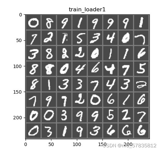
图像的真实标签:
0 8 9 1 9 9 9 1
7 2 1 5 3 4 0 7
3 8 2 2 0 1 1 6
8 8 0 4 6 4 7 5
8 1 3 3 7 4 3 2
7 9 7 2 0 6 1 6
0 0 3 9 9 5 2 7
0 3 1 9 3 6 6 6
- 在network4.py定义一个卷积神经网络,即Transfer类,该类与之前训练的MNIST手写数字识别模型的卷积层一样。当输入两张图像,构造两个并行的卷积层,提取两张图像的特征。然后将图象特征放入全连接层,因为10种数字图像的和一共有19种结果,所以最终全连接输出层设置为19个单元。
- 将之前训练的MNIST手写数字识别模型导出,这里导出的模型保存为model_new902,在network4.py中编写show_testset_total_accuracy(model:str)函数,来测试该导出模型的准确率。在network4.py运行该函数,结果如下:
ConvNet(
(conv1): Conv2d(1, 6, kernel_size=(5, 5), stride=(1, 1), padding=(2, 2))
(pool): MaxPool2d(kernel_size=2, stride=2, padding=0, dilation=1, ceil_mode=False)
(conv2): Conv2d(6, 16, kernel_size=(5, 5), stride=(1, 1), padding=(2, 2))
(fc1): Linear(in_features=784, out_features=512, bias=True)
(fc2): Linear(in_features=512, out_features=10, bias=True)
)
model_new902模型在测试集上的准确率:99.22%
可以看到准确率达到99%。该模型已经很好了。
- 我们先在不依靠之前训练的模型的情况下,在仅有2000张的图像的训练集下,训练这个加法器网络,观察在多少轮达到多高的测试集准确率。这里在network4.py中编写cycle_training(net,num_epochs=20)函数,该函数里定义一个损失函数和优化器,使用分类交叉熵Cross-Entropy 作损失函数,动量SGD做优化器,对不依赖模型的加法器网络进行训练。在main.py文件中调用该方法即可,得运行结果:
…
训练周期: 19 [1536/2000 (78%)] 训练误差:1.90 校验误差:2.00 训练准确率:28.75% 验证准确率:26.56%
训练周期: 19 [1856/2000 (94%)] 训练误差:1.90 校验误差:1.98 训练准确率:25.62% 验证准确率:26.86%
最终测试集准确率:33.72%

-
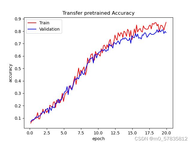
我们接下来迁移之前训练的模型,先在network4.py文件中定义Transfer类的set_filter_values(self, net)方法,该方法的作用是将迁移过来的网络的权重值拷贝到本网络中去,接着在network4.py文件中定义cycle_training_to_transfer_pretrained(net,original_net,num_epochs=20)函数,该函数在迁移的情况下,同在仅有2000张的图像的训练集下,训练这个加法器网络(这里只是把之前网络模型的卷积层权值迁移过来,并没有固定,之后训练,随梯度下降,而更新权值),我们可观察在多少轮达到多高的测试集准确率。同样在main.py文件中调用该方法即可,得运行结果:
…
训练周期: 19 [1536/2000 (78%)] 训练误差:0.47 校验误差:0.66 训练准确率:84.38% 验证准确率:79.82%
训练周期: 19 [1856/2000 (94%)] 训练误差:0.45 校验误差:0.69 训练准确率:87.19% 验证准确率:78.96%
最终测试集准确率:88.14%
-
我们也是迁移之前训练的模型,先在network4.py文件中定义Transfer类的set_filter_values_nograd(self,
net)方法,该方法的作用是将迁移过来的网络的权重值拷贝到本网络中去,并且迁移为固定权重式,接着在network4.py文件中定义cycle_training_to_transfer_fixed(net,original_net,num_epochs=20)函数,该函数在迁移的情况下,同在仅有2000张的图像的训练集下,训练这个加法器网络(这里把之前网络模型的卷积层权值迁移过来,并且固定下来,之后训练不在更新权值,只改改变全连接层的权值),我们可观察在多少轮达到多高的测试集准确率。同样在main.py文件中调用该方法即可,得运行结果:…
训练周期: 19 [1536/2000 (78%)] 训练误差:0.87 校验误差:0.85 训练准确率:71.25% 验证准确率:73.32%
训练周期: 19 [1856/2000 (94%)] 训练误差:0.86 校验误差:0.87 训练准确率:74.38% 验证准确率:73.22%
最终测试集准确率:82.92%

-
最后在network4.py文件中定义show_different_network_training_result(r0,r1,r2)函数,该函数展示以上不同策略训练的网络的结果,即可视化不同方式训练的加法器网络的效果,对比验证“迁移学习是否可以将在一个领域训练的机器学习模型应用到另一个领域,在某种程度上是否提高了训练模型的利用率,能否解决了数据缺失的问题,并赋予了智能模型“举一反三”的能力“。在main.py中将以上训练结果作为参数,调用。得到结果:
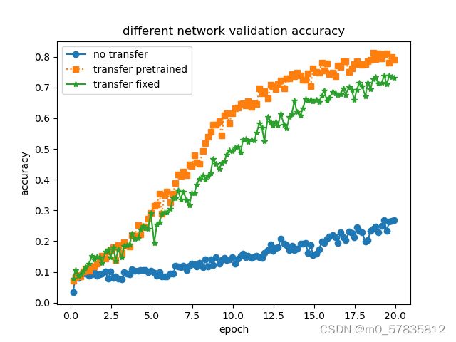
在没有迁移的加法器网络上,因为训练集只有2000张图片,即使训练轮数达到20轮之多,在验证集上的准确率都不过30%.而迁移了模型的加法器网络,在随着训练轮数的增加,准确率在提升。而固定了的迁移模型略逊于没有固定的迁移模型,这可能是因为之前训练模型的训练集与该训练集的整体特征不太相符,而固定了的模型,没有改进提取特征的能力。
总结
选择一个合适的模型去训练特定任务,发挥预训练模型特征抽象的能力,通过微调,改变它的部分参数或者为其新增部分输出结构后,在小部分数据集上训练,来使整个模型更好的适应特定任务。但在选用预训练模型是小型模型的情况下,可以通过增加训练次数来提高效果。