【目标跟踪】基于UKF、EKF、PF实现目标跟踪matlab代码
1 简介
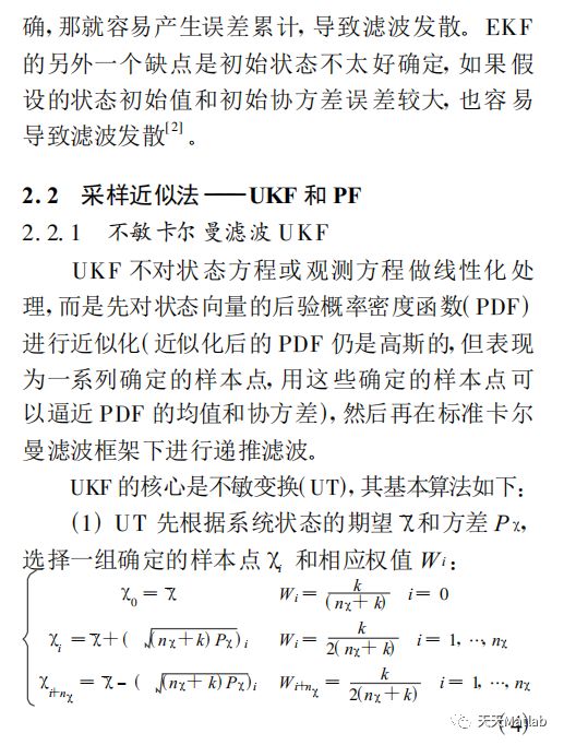
雷达系统的非线性目标跟踪已被人们广泛重视。扩展卡尔曼滤波器(EKF)是将卡尔曼滤波器(KF)局部线性化,其算法简单、计算量小,适用于弱非线性、高斯环境下。不敏卡尔曼滤波器(UKF)是用一系列确定样本来逼近状态的后验概率密度,在高斯环境中,对任何非线性系统都有较好的跟踪性能。粒子滤波器(PF)是用随机样本来近似状态后验概率密度函数,适用于任何非线性非高斯系统。文中通过仿真实验,对三者的性能进行了仿真比较,结果证明在复杂的非高斯非线性环境中,粒子滤波器的性能明显优于另外两种滤波器,但计算复杂,耗时长。
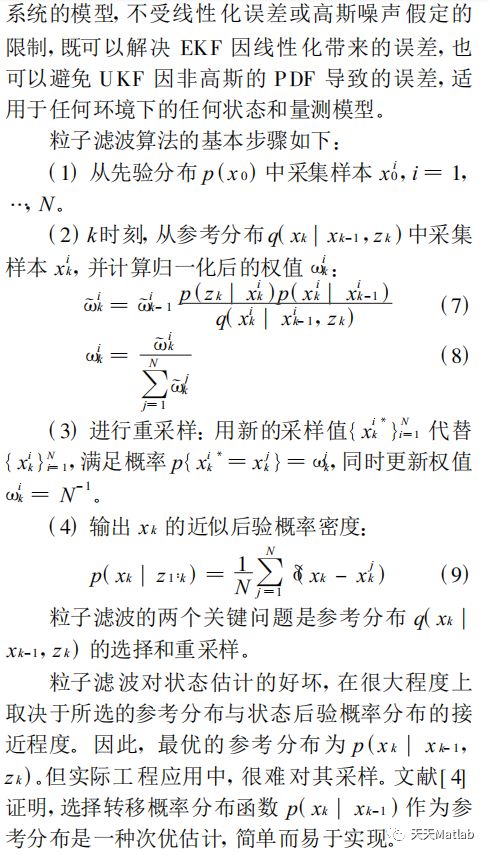
通常 ,对于雷达系统下的数据处理 ,目标的状 态方程是在直角坐标系下描述的, 而量测方程是 在极坐标或球坐标下得到的 , 因而在同一坐标系 下研究状态方程和量测方程不可能都是线性的。 这样 ,雷达数据处理中的目标跟踪面临着非线性滤波问题 。 为了实现最优非线性滤波, 需要得到目标状 态后验概率密度函数的完整描述。然而 ,在实际 的雷达跟踪中这是很难得到的。为此, 人们提出 了大量次优的近似估计方法 。本文中我们将讨论两类三种非线性滤波技术。一类是函数近似法 。 函数近似法是对非线性的状态方程或观测方程作 线性化处理 , 典型的 算法 是扩 展卡尔 曼滤 波 (EKF)。 EKF 先利用泰勒展开的一次项来对非线 性方程作线性化处理, 再结合经典的卡尔曼滤波 进行滤波估计。 EKF 算法简单 ,易于实现 ,但在强非线性和非高斯环境下跟踪性能较差, 甚至会出 现滤波发散;另一类是基于采样方法的近似法 。 采样近似法用带有权值的样本集来近似目标的状态后验概率密度(PDF),典型的算法有不敏卡尔曼滤波(UKF)和粒子滤波(PF), 其中 UKF 采用的 是确定的样本点 ,因而避免了由线性化而导致的跟踪误差 ,但当状态的后验概率密度是非高斯时, 跟踪性能会随之下降。而 PF 采用的是空间随机样本 ,它独立于系统的模型, 与模型是否线性 、是否高斯无关,因此, 粒子滤波可应用在各种系统模型下 。


2 部分代码
% Main file for first geolocation simulation: isotropic static jammer
% -----------------------------------------------------------------------
% ------------------------ Algorithm ------------------------------
% -----------------------------------------------------------------------
% The algorithm goes through: prompts & constants, simulation parameters,
% variable initialisation, main loop, error checking and plotting
% There are two distinct parts: the flyby section and the orbital
% adaptation main loop uses simple Euler integration to update the UAV
% dynamics and it updates filter parameters
% Matrices (or vectors) are in column form that is each new entry forms a
% new line i.e: A(k+1,:)=...
% WARNING: THE ONLY EXCEPTIONS are filters' states which are in line form
% i.e: A(:,k+)=...
% The floor function is used to get a integer out of a percentage of
% another integer e.g floor((5/100)*N_loops_fb): integer of 5/100 of total
% number of iterations of the simulation
% The rem (remainder) function is used to know if a number divided by
% another is an integer (Euclidian division)
% Workspace cleaning
clc; close all; clear all;
global d2r
% Constants (not to be modified)
d2r=pi/180; % Value in rad = Value in deg * d2r
r2d=1/d2r; % Value in deg = Value in rad * r2d
g_0=9.81; % Gravity acceleration assumd constant [m/s^2]
f_L1=1575.42*10^6; % L1 frequency [Hz]
c_0=299792458; % speed of light [m/s]
k_b=1.3806488*(10^(-23)); % Boltzmann constant
%%
% -----------------------------------------------------------------------
% -------------------- Simulation parameters ----------------------
% -----------------------------------------------------------------------
% Parameters (Simulation design): Change according to desired simulation
% Within the simulation, these are fixed
% Area parameters and number of iterations are global variables
global x_bnd y_bnd N_loops_fb
% Simulation parameters
D_T=1/2; % Sampling time of the simulation (for Euler integration) [s] - half a second is fine for filter accuracy and animation speed
t_0=0; % Initial time [s]
t_f_fb=4.5*60; % Final time for flyby [s] - Check with speed to know what distance will be travelled - 6 minutes at 30m/s is fine for straight flyby
t=(t_0:D_T:t_f_fb-t_0)'; % Time vector for flyby [s]
N_loops_fb=size(t,1); % Number of loops in the flyby simulation
t_f_vf=15*60; % Final time for the Vector field part. Note it is not its duration but the time at which it stops
t=(t_0:D_T:t_f_vf-t_0)'; % Time vector for whole simulation
N_loops_vf=size(t,1); % Total number of loops for the simulation
% Search Area parameters
x_bnd=12*10^3; % x area boundary [m]
y_bnd=12*10^3; % y area boundary [m]
A_area=x_bnd*y_bnd; % Area of search [m瞉
% Jammer parameters
% Static Jammer true location : located within a square centred
% inside the search area. These parameters are not known by the UAV
x_t_vec=place_jammer(); % See corresponding function. It places the jammer randomly in a square in the search area
% GPS jammer model for the simulation
P_t_min=1*(10^(-3)); % [W] - Generally around 1mW
P_t_max=650*(10^(-3)); % [W] - Generally 650mW
% Jammer power in the L1 band: to be adjusted for desired
% simulation. Assumed always constant (civil jammers)
% Jammer orientation
psi_jammer=0; % Degrees [0-360]
psi_jammer=psi_jammer*d2r; % In radians
% Jammer Gain distribution
% Load data: azimvals,elevvals and gainvals that are used in
% the simulink 'lookup' file
load('Ducati_jam2_LHCP.mat');
% Jammer power
P_t=(P_t_min+(P_t_max-P_t_min)*rand(1,1)); % Power [W] - Line to comment if the user wants to specify a given power within power bounds
% Display jammer power as it is an important simulation parameter
P_t_jammer_str=num2str(P_t*(10^3)); % convert to mW, then to string for display
disp('--> GPS jammer Power in L1 band for this simulation is :'); % display
disp([P_t_jammer_str,' mW']); % display
% Jammer gain
G_t=1; % Isotropic, lossless antenna []
% Jammer sweep range: [f_L1-f_min ; f_L1+f_max]
f_min=f_L1-30*10^6; % [Hz] - f_min and f_max around 10-20-30 MHz
f_max=f_L1+30*10^6; % [Hz]
% UAV parameters
% Initial position and heading
[x_vec psi_0]=place_uav();% See corresponding function. It places the UAV randomly in a small square in the South-West area with a random heading
% Altitude-hold
h_0=125; % Constant altitude of the UAV [m]
% UAV airspeed
V_g=28.3; % Average Cruising Airspeed of the aerosonde [m/s]
V_min=15; % Minimum safe speed [m/s]
V_max=50; % Maximum safe speed [m/s]
% UAV minimum turn radius
min_turn_r=200; % Minimum safe turn radius [m]
% UAV Antenna Gain
G_r=1; % Isotropic, lossless antenna []
% Obtain side on which the jammer lies:
% port of UAV--> true_side=1 starboard of UAV--> true_side=0
true_side=get_true_side(x_t_vec,x_vec,psi_0); % See corresponding function for details
% UAV path parameters: the winding path is generated by cosinusoidal
% heading command (psi-psi_0)=psi_range*cos((2pi/dist_period)*distance_travelled)
dist_period=(10/4)*10^3; % Distance travelled by UAV during one winding path period [m]
psi_range=(2*pi/4); % Psi variation range during winding path [rad]
% Measurement process parameters
% Friis' equation constant parameter called gamma_0
gamma_0=G_t*G_r*((c_0/(4*pi*f_L1))^2); % Coefficient assumed constant
% Measurement noise
Temperature=23; % Temperature of the sensor [C癩
P_thermal_noise=k_b*(Temperature+273.15)*abs(f_max-f_min); % Thermal noise using Johnson朜yquist equation
P_thermal_noise_dBm=10*log10(1000*P_thermal_noise); % Converstion in dBm
% Filtering
low_pass_freq=0.06; % Low pass filter cut-off frequency W_n: check help butter for more information (good values 0.01 - 0.1)
butter_order=2; % Order of the low-pass filter generated by the butterworth command
[b_butter,a_butter]=butter(butter_order,low_pass_freq); % Obtain Butterworth filter coefficients
% Sensor power measurement standard deviation: Choose and disable
% lines for noise specification or for thermal noise approximation:
sig_P_r=-120; % Gaussian noise affects Power measurement P_r: std sigma in [dBm]
%sig_P_r=3*P_thermal_noise_dBm; % std sigma based on thermal noise [dBm]
%sig_P_r_W=P_thermal_noise/3; % std sigma based on thermal noise [W]
sig_P_r_W=((10^(sig_P_r/10))/1000); % std sigma in [W]
% Geolocation process parameters
% Confidence interval/max band for received power peak determination
conf_intvl=(1-(2/100)); % Default setting: 2%
k_H_g=0; % Serves as a check condition on the passing of a minimum distance to the jammer for straight flyby
P_r_filt_max=0; % Initialise maximum filtered power received. Serves as check condition for max determination for straight flyby
band_found=0; % Serves as boolean to check whether the max band has been found straight flyby
% Extended Kalman filtering based on alpha-measurements
% Parameters for filter start
k_C_prim=floor((0.5/100)*N_loops_fb)+1; % Initialise k_C_prim: step used to determine whether two circles seperated by a given distance intersect
obs_check=0; % Boolean parameter for filter start: initialise start as false
k_obs=1; % Step at which obs_check turns true
div_EKF_bool=0; % Boolean for filter track divergence: initialise as false
% filter initialisation:
F_KF=eye(2); % Dynamics matrix: unity because model is static
G_KF=eye(1); % Noise matrix: unity for pure additive gaussian noise
%%%%%%%%%%%%%%%%%%%%%%%%%%%%%%%%%%%%%%%%%%%%%%%%%%%%%%%%%%%%%%%
%---------- < Q_KF must be set up appropriately > ------------%
%%%%%%%%%%%%%%%%%%%%%%%%%%%%%%%%%%%%%%%%%%%%%%%%%%%%%%%%%%%%%%%
Q_KF=diag([((0.01))^2 ((0.1))^2]); % Process noise matrix: better to be small std for position and power
%%%%%%%%%%%%%%%%%%%%%%%%%%%%%%%%%%%%%%%%%%%%%%%%%%%%%%%%%%%%%%%
%%%%%%%%%%%%%%%%%%%%%%%%%%%%%%%%%%%%%%%%%%%%%%%%%%%%%%%%%%%%%%%
%%%%%%%%%%%%%%%%%%%%%%%%%%%%%%%%%%%%%%%%%%%%%%%%%%%%%%%%%%%%%%%
%%%%%%%%%%%%%%%%%%%%%%%%%%%%%%%%%%%%%%%%%%%%%%%%%%%%%%%%%%%%%%%
%---------- < Q_KF must be set up appropriately > ------------%
%%%%%%%%%%%%%%%%%%%%%%%%%%%%%%%%%%%%%%%%%%%%%%%%%%%%%%%%%%%%%%%
R_KF=(2).^2; % Specify noise on alpha: enable if wanted
%%%%%%%%%%%%%%%%%%%%%%%%%%%%%%%%%%%%%%%%%%%%%%%%%%%%%%%%%%%%%%%
%%%%%%%%%%%%%%%%%%%%%%%%%%%%%%%%%%%%%%%%%%%%%%%%%%%%%%%%%%%%%%%
%%%%%%%%%%%%%%%%%%%%%%%%%%%%%%%%%%%%%%%%%%%%%%%%%%%%%%%%%%%%%%%
x_state_ini=[x_bnd/2 1*y_bnd/2]'; % Initial state guess - Middle of the area is the first guess
%%%%%%%%%%%%%%%%%%%%%%%%%%%%%%%%%%%%%%%%%%%%%%%%%%%%%%%%%%%%%%%
%---------- < Q_KF must be set up appropriately > ------------%
%%%%%%%%%%%%%%%%%%%%%%%%%%%%%%%%%%%%%%%%%%%%%%%%%%%%%%%%%%%%%%%
P_cov_ini=diag([sqrt(4000)^2 sqrt(4000)^2]); % Initial state covariance guess - Change if needed
%%%%%%%%%%%%%%%%%%%%%%%%%%%%%%%%%%%%%%%%%%%%%%%%%%%%%%%%%%%%%%%
%%%%%%%%%%%%%%%%%%%%%%%%%%%%%%%%%%%%%%%%%%%%%%%%%%%%%%%%%%%%%%%
%%%%%%%%%%%%%%%%%%%%%%%%%%%%%%%%%%%%%%%%%%%%%%%%%%%%%%%%%%%%%%%
% Parameters for fiter rerun
re_run_bool=0;
% Vector field part parameters
% Desired radius r_d for the orbit around the jammer
r_d=1000; % in metres [m]
alpha_f=1; % Normalising constant on V_g during orbital adaptation: alpha=1 --> V=V_g
K_LVFG_psi=3.0; % Gain on the heading rate command for the LVFG
% Prepare plot for animation
global plot_scaling fig_offset
% Plot parameters
N_plots=1; % Counter for plots
plot_scaling=10^3; % IMPORTANT: Scale to kilometers --> Changing this parameter will need changing axes labels
fig_offset=1/100; % Area offset to figure boundaries [% of bounds x_bnd & y_bnd]
p_e=95/100; % Confidence probability for the error covariance based on P_cov
%%
% -----------------------------------------------------------------------
% ------ Initialise simulation parameters for flyby phase ----------
% -----------------------------------------------------------------------
% UAV
x_vec_all=zeros(N_loops_fb,2); % Initialise uav position vector
x_vec_all(1,:)=x_vec; % idem for initial postion
x_vec_dot=zeros(N_loops_fb,2); % Initialise uav velocity vector: derivative of x_vec_all
psi_all=zeros(N_loops_fb,1); % Initialise uav heading vector
psi_all(1,:)=psi_0; % Idem for initial heading
psi_dot=zeros(N_loops_fb,1); % Initialise uav heading derivative vector
jammer_UAV_vec_p=zeros(N_loops_fb,3); % Initialise Jammer-->UAV vector (3D)
elev_angle=zeros(N_loops_fb,1); % Initialise elevation angle to vertical
azimuth_angle=zeros(N_loops_fb,1); % Initialise jammer-->UAV azimuth angle to horizontal
azimuth_rel_angle=zeros(N_loops_fb,1); % Initialise jammer-->UAV azimuth angle to jammer direction
% Measurements
r_true=zeros(N_loops_fb,1); % True slant range
P_r_true=zeros(N_loops_fb,1); % True received power
P_r_meas=zeros(N_loops_fb,1); % Measured received power: with noise
G_t_sim_sto=zeros(N_loops_fb,1); % Store every Jammer gain
% Processing
r_est_l=zeros(N_loops_fb,1); % Lower range estimation
r_est_h=zeros(N_loops_fb,1); % Upper range estimation
r_est_unc=zeros(N_loops_fb,1); % Range estimation uncertainty
P_r_filt_ratio=zeros(N_loops_fb,1); % Alpha: Power ratio between initial and current : see 'alpha' in report
centre_geo_circle=zeros(N_loops_fb,2); % Centre of geolocation circle at instant k
radius_geo_circle=zeros(N_loops_fb,1); % Radius of geolocation circle at instant k
% Filters
%
x_state=zeros(2,N_loops_fb); % Updated filter state vector for all steps
P_cov=zeros(2,2,N_loops_fb); % filter Covariance matrix for all
K_EKF_gain=zeros(2,N_loops_fb); % Kalman gain storage
% Simulation data
d_uav=zeros(N_loops_fb,1); % Distance travelled by the UAV
%%
% -----------------------------------------------------------------------
% ------------------ Main flyby simulation Part --------------------
% -----------------------------------------------------------------------
ave begun & filter has alreay started
%%%%%%%%%%%%%%%%%%%%%%%%%%%%%%%%%%%%%%%%%%%%%%%%%%%%%%%%%%%%%%%
%-------- < check the performance of the EKF (UKF) > ---------%
%------------- < Design a new filer algorithm > --------------%
%%%%%%%%%%%%%%%%%%%%%%%%%%%%%%%%%%%%%%%%%%%%%%%%%%%%%%%%%%%%%%%
% To make sure this file run, I just put x_state(:,k) = x_t_vec
% (the true target postion)
%x_state(:,k) = x_t_vec;
%%% students must uncomment the following line and design a new
%%% fitler anglrithm to alleviate the peformance degradation
%%% casued by anisotropic jammer pattern
[x_state(:,k),P_cov(:,:,k),K_EKF_gain(:,k)]=UKF_form(x_vec_all(1,:),x_vec_all(k,:),h_0,P_r_filt_ratio(k,1),x_state_ini,P_cov_ini,F_KF,G_KF,Q_KF,R_KF,G_t_sim_sto(1,1),G_t_sim_sto(k,1));
end
% filter RMS calculation and P_t estimation
% Animation: plot new UAV, Jammer and UAV trace at each iteration.
% See corresponding function for detail
plot_animation_search(N_plots,k,x_t_vec,x_vec_all(1:k,:),psi_all(k,1),r_est_l(k,1),r_est_h(k,1),centre_geo_circle(k,:),radius_geo_circle(k,1),x_state(:,1:k),k_obs,N_loops_fb,P_cov(:,:,k),p_e,0,psi_jammer);
end
% ------------------------ End Main flyby loop -----------------------------
%%
% -----------------------------------------------------------------------
% ------------------- Flyby Results Analysis -----------------------
% -----------------------------------------------------------------------
%%%%%%%%%%%%%%%%%%%%%%%%%%%%%%%%%%%%%%%%%%%%%%%%%%%%%%%%%%%%%%%
%%%% Students must analyse the performance of their own filters
%%%%%%%%%%%%%%%%%%%%%%%%%%%%%%%%%%%%%%%%%%%%%%%%%%%%%%%%%%%%%%%
%%
% -----------------------------------------------------------------------
% -- Initialise Vector field simulation parameters from flyby phase -
% -----------------------------------------------------------------------
% This part consists in augmenting previous matrices from flyby with
r_est_l=[r_est_l ; zeros(N_loops_vf-N_loops_fb,1)]; % Lower range estimation
r_est_h=[r_est_h ; zeros(N_loops_vf-N_loops_fb,1)]; % Upper range estimation
r_est_unc=[r_est_unc ; zeros(N_loops_vf-N_loops_fb,1)]; % Range estimation uncertainty
P_r_filt_ratio=[P_r_filt_ratio ; zeros(N_loops_vf-N_loops_fb,1)]; % Alpha: Power ratio between initial and current : see 'alpha' in report
centre_geo_circle=[centre_geo_circle ; zeros(N_loops_vf-N_loops_fb,2)]; % Centre of geolocation circle at instant k
radius_geo_circle=[radius_geo_circle ; zeros(N_loops_vf-N_loops_fb,1)]; % Radius of geolocation circle at instant k
% Filters
% filter
r_est=zeros(N_loops_vf,1); % Only used in the second part (VF)
x_state=[x_state zeros(2,N_loops_vf-N_loops_fb)]; % Updated filter state vector for all steps
P_cov(:,:,N_loops_fb+1:N_loops_vf)=0; % filter Covariance matrix for all
K_EKF_gain=[K_EKF_gain zeros(2,N_loops_vf-N_loops_fb)]; % Kalman gain storage
% Simulation data
d_uav=[d_uav ; zeros(N_loops_vf-N_loops_fb,1)]; % Distance travelled by the UAV
d_uav(N_loops_fb+1,1)=d_uav(N_loops_fb,:)+D_T*sqrt(x_vec_dot(N_loops_fb,:)*(x_vec_dot(N_loops_fb,:))');
% Get Vector field orientation depending on UAV heading and azimuth to
% jammer
psi_uav=rem(psi_all(N_loops_fb,1),2*pi); % UAV heading (0 - 2pi)
beta_angle=psi_uav-azimuth_angle(N_loops_fb,1); % Angle between Jammer-->UAV and UAV heading
beta_angle = rem(beta_angle,2*pi); % psi_diff in [0 2*pi]
if abs(beta_angle)>pi
beta_angle = beta_angle-2*pi*sign(beta_angle);
end
if (beta_angle>=0)
VF_rot_sen=1; % Counter-clockwise
else
VF_rot_sen=-1; % Clockwise
end
%%
% -----------------------------------------------------------------------
% ------ Main Vector Field (VF) simulation Part --------------
% -----------------------------------------------------------------------
% UAV movement:
if k~=N_loops_vf % Not updated past (N_loops_vf-1)
x_vec_all(k+1,:)=x_vec_all(k,:)+D_T*x_vec_dot(k,:); % Position Euler integration
psi_all(k+1,:)=psi_all(k,:)+D_T*psi_dot(k,:); % Heading Euler integration
d_uav(k+1,:)=d_uav(k,:)+D_T*sqrt(x_vec_dot(k,:)*(x_vec_dot(k,:))'); % Travelled distance Euler integration
end
% UAV true attitude toward jammer (azimuth (0 2pi) relative to x-axis and
% elevation (0 - pi) relative to z-axis: spherical coordinates)
jammer_UAV_vec_p(k,1:2)=x_vec_all(k,:)-x_t_vec; % Obtain 2D jammer-->UAV vector
jammer_UAV_vec_p(k,3)=h_0; % Augment with third dimension: altitude
jammer_UAV_vec_p(k,:)=(jammer_UAV_vec_p(k,:)/(sqrt(jammer_UAV_vec_p(k,:)*(jammer_UAV_vec_p(k,:)')))); % Normalise vector
elev_angle(k,1)=acos(jammer_UAV_vec_p(k,:)*([0 0 1]')); % Get elevation angle theta using dot product [rad]
azimuth_angle(k,1)=atan2(jammer_UAV_vec_p(k,2),jammer_UAV_vec_p(k,1)); % Azimuth angle (-pi pi)
if (0>azimuth_angle(k,1)>=-pi)
azimuth_angle(k,1)=2*pi+azimuth_angle(k,1);
end
azimuth_angle(k,1)=rem(azimuth_angle(k,1),2*pi);
azimuth_rel_angle(k,1)=azimuth_angle(k,1)-psi_jammer;
if ((0>azimuth_rel_angle(k,1))&&(azimuth_rel_angle(k,1)>=-2*pi))
azimuth_rel_angle(k,1)=2*pi+azimuth_rel_angle(k,1);
end
% Continually check for UAV out of boundaries
if ((x_vec_all(k,1)<2*min_turn_r)||(x_vec_all(k,1)>(x_bnd-2*min_turn_r))||(x_vec_all(k,2)<2*min_turn_r)||(x_vec_all(k,2)>(y_bnd-2*min_turn_r)))
disp('UAV is going out of boundaries when it should not.')
disp('Simulation stops. Check guidance for troubleshooting')
return % Stop simulation if this happens
end
% Gain of the jammer (recall assumption G_r=1 ) from the azimuth and
% elevation angles
sim('look_up_aid_w_ducati'); % Jammer gain interpolation
G_t=G_t_sim;
G_t_sim_sto(k,1)=20*log10(G_t_sim);
% UAV measurement:
r_true(k,1)=sqrt(((x_vec_all(k,1)-x_t_vec(1,1))^2)+((x_vec_all(k,2)-x_t_vec(1,2))^2)+(h_0^2));
% True Received power through Friis equation. However f varies
% slightly and the instrumentation measures P_r with some error
P_r_true(k,1)=(P_t*G_t*G_r*((c_0/(4*pi*r_true(k,1)*f_L1))^2)); % Equation 3.6 in report: Friis P_r in [W]
P_r_meas(k,1)=P_r_true(k,1)+sig_P_r_W*randn(1); % Add noise in W
% UAV measurement pre-processing
% Received power filtering
if (k>3*butter_order) % filter only works with sufficient data points
P_r_filt=zeros(k,1); % Re-Initialise filtered data at each step
P_r_filt(1:k,1)=filtfilt(b_butter,a_butter,P_r_meas(1:k,1)); % Filter noisy P_r_true at each new step
end
% Simulation data:
% Process measurements for geolocation
% First: process range determination
if (k>3*butter_order) % If simulation has enough point (filtering)
r_est_l(k,1)=((c_0/(4*pi*f_L1))*sqrt((G_t*G_r/(P_r_filt(k,1)))*P_t_min)); % Evaluate lower range from measurements
r_est_h(k,1)=((c_0/(4*pi*f_L1))*sqrt((G_t*G_r/(P_r_filt(k,1)))*P_t_max)); % Evaluate Upper range from measurements
r_est_unc(k,1)=abs(r_est_h(k,1)-r_est_l(k,1)); % Evaluate uncertainty on range measurements
end
% Second: process iso-(range ratio) curves
if (k>3*butter_order+1) % If simulation has initialised
P_r_filt_ratio(k,1)=((P_r_filt(k,1)))/(P_r_filt(1,1)); % Get power ratio: alpha
if (abs((P_r_filt_ratio(k,1)-1))>0.05/100) % If ratio away from 1 with confidence
[centre_geo_circle(k,:) radius_geo_circle(k,1)]=get_geo_data(x_vec_all(1,:),x_vec_all(k,:),P_r_filt_ratio(k,1)); % See corresponding function
else
alpha_eq_1=1; % Boolean to indicate that ratio is close to 1 therefore set to 1 in the simulation
end
end
% filtering
if (re_run_bool==1) % If filter has diverged and needs to reinitialised
%%%%%%%%%%%%%%%%%%%%%%%%%%%%%%%%%%%%%%%%%%%%%%%%%%%%%%%%%%%%%%%
%-------- < check the performance of the EKF (UKF) > ---------%
%------------- < Design a new filer algorithm > --------------%
%%%%%%%%%%%%%%%%%%%%%%%%%%%%%%%%%%%%%%%%%%%%%%%%%%%%%%%%%%%%%%%
% To make sure this file run, I just put x_state(:,k) = x_t_vec
% (the true target postion)
%x_state(:,k) = x_t_vec;
%%% students must uncomment the following line and design a new
%%% fitler anglrithm to alleviate the peformance degradation
%%% casued by anisotropic jammer pattern
[x_state(:,k),P_cov(:,:,k),K_EKF_gain(:,k)]=UKF_form(x_vec_all(1,:),x_vec_all(k,:),h_0,P_r_filt_ratio(k,1),x_state_ini,P_cov_ini,F_KF,G_KF,Q_KF,R_KF,G_t_sim_sto(1,1),G_t_sim_sto(k,1));
re_run_bool=0;
div_EKF_bool=0;
elseif (re_run_bool==0) % Normal operation condition: the filter has converged and remains on target
%%%%%%%%%%%%%%%%%%%%%%%%%%%%%%%%%%%%%%%%%%%%%%%%%%%%%%%%%%%%%%%
%-------- < check the performance of the EKF (UKF) > ---------%
%------------- < Design a new filer algorithm > --------------%
%%%%%%%%%%%%%%%%%%%%%%%%%%%%%%%%%%%%%%%%%%%%%%%%%%%%%%%%%%%%%%%
% To make sure this file run, I just put x_state(:,k) = x_t_vec
% (the true target postion)
%x_state(:,k) = x_t_vec;
%%% students must uncomment the following line and design a new
%%% fitler anglrithm to alleviate the peformance degradation
%%% casued by anisotropic jammer pattern
[x_state(:,k),P_cov(:,:,k),K_EKF_gain(:,k)]=UKF_form(x_vec_all(1,:),x_vec_all(k,:),h_0,P_r_filt_ratio(k,1),x_state_ini,P_cov_ini,F_KF,G_KF,Q_KF,R_KF,G_t_sim_sto(1,1),G_t_sim_sto(k,1));
end
% Animation: plot new UAV, Jammer and UAV trace at each iteration.
% See corresponding function for detail
plot_animation_search(N_plots,k,x_t_vec,x_vec_all(1:k,:),psi_all(k,1),r_est_l(k,1),r_est_h(k,1),centre_geo_circle(k,:),radius_geo_circle(k,1),x_state(:,1:k),k_obs,N_loops_fb,P_cov(:,:,k),p_e,r_d,psi_jammer);
end
%%
% -----------------------------------------------------------------------
% ------------------------ Performance Check -------------------------
% -----------------------------------------------------------------------
%%%%%%%%%%%%%%%%%%%%%%%%%%%%%%%%%%%%%%%%%%%%%%%%%%%%%%%%%%%%%%%
%%%% Students must analyse the performance of their own filters
%%%%%%%%%%%%%%%%%%%%%%%%%%%%%%%%%%%%%%%%%%%%%%%%%%%%%%%%%%%%%%%
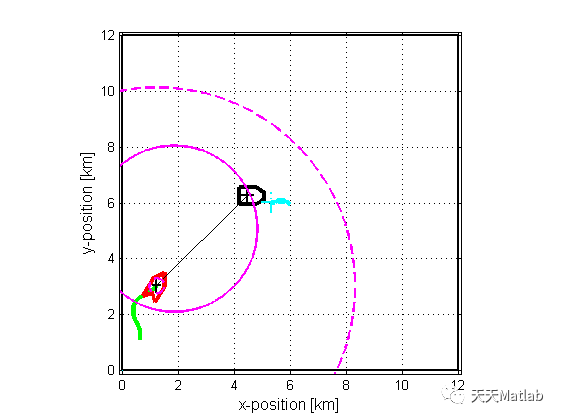
3 仿真结果


4 参考文献
[1]万莉, 刘焰春, and 皮亦鸣. "EKF、UKF、PF目标跟踪性能的比较." 雷达科学与技术 01(2007):13-16.
