CS231n KNN笔记

CS231n KNN笔记

1.参考课程笔记翻译

KNN上 , KNN下

2.笔记内容摘录

2.1.最近邻和K-近邻思想简述

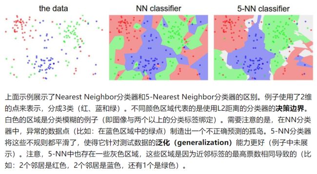
1. 最近邻（Nearest Neighbor）是寻找与当前测试图像的像素差异最近的一张训练图像，并以找到的训练图像的类别作为测试图像的类别。这里的像素差异又被称为距离，关于这个距离的定义有很多种，也就是属于超参数。
2. K-近邻是寻找寻找与当前测试图像的像素差异最近的K张训练图像，并且以这些图像中类别数最多的那个分类作为测试图像的类别。这样就提高了可信度，减小异常数据点的干扰。但是也存在问题，就是可能K张图像中有两类或几类的图像数相等， 这时候分类就存在灰色区域。

2.2准确率

Yte_predict = nn.predict(Xte_rows) # 输入测试集，得到预测的分类标签
print 'accuracy: %f' % ( np.mean(Yte_predict == Yte) )
# 1.Yte_predict == Yte 得到一个bool类型的数组，如果预测正确值为True,也就是1
# 2.np.mean求这个数组的平均值，也就是最后的准确率

2.3.xrange和range

简单说说range和xrange的区别

1. 这是课程官方为了兼容Python2和python3的操作
2. 只有在python2中才有xrange和range，python3中没有xrange，并且python3中的range和python2中的range有本质的区别。所以这儿说的range和xrange的区别是只针对python2的

• 不同点

  • range : 在py2中，range得到的是一个列表,即

      x = range(0, 5)
      print(type(x))  # 打印x的类型，结果是list
      print(x) # 结果是[0,1,2,3,4]
  

  • xrange ：在py2中，xrange得到的是一个生成器对象， 即

      x = xrange(0, 5)
      print(type(x))  # 输出类型，结果为一个生成对象
      print(x)  # 输出x， 结果为xrange(0,5)
  

  那么，python3中为什么没有了range了呢（额，这个怎么描述呢，是有range，但是这个range其实是py2中的xrange，而不是range），因为使用生成器可以节约内存。比如现在有个代码是for i in range(0, 10000)，如果还是使用py2中的range的话，那你就会得到一个0到9999的一个列表，这个将会占用你很大的空间，但是使用生成器的话，就会节省很大的资源。

• 共同点

  它们的使用都是一样的，比如都可以用for循环遍历所有的值

2.4.计算距离

1. L1距离

   """ X is N x D where each row is an example we wish to predict label for """
   distances = np.sum(np.abs(self.Xtr - X[i,:]), axis = 1)
   min_index = np.argmin(distances) 
   Ypred[i] = self.ytr[min_index] 
   

   • X是输入的测试集，每一行都是一张图片展开的行向量，np.abs(self.Xtr - X[i,:])就是计算第i张图片和所有测试集的距离，在减法运算过程中对测试机的第i行的行向量进行了广播，然后np.abs求绝对值。
   • np.sum(xx, axis=1)是针对上面求得的L1距离，对每一行求和，得到的就是第i张图片和所有的训练集的L1距离。
   • np.argmin(distances)寻找L1距离最小的训练集的索引，也就是和测试图片最相似的训练集图片。
   • Ypred[i] = self.ytr[min_index]得到这个图片的分类标签。

2. L2距离

   distances = np.sqrt(np.sum(np.square(self.Xtr - X[i,:]), axis = 1))
   

   具体计算步骤同上。

3. 关于L1距离和L2距离的区别

   TODO

2.5.超参数调优

1. 最后一步、且仅使用一次测试集
2. 从训练集中分出一部分数据用做验证集，用来进行超参数调优
3. 训练集数据不够时，验证集数据更少，这时候可以将训练集均分成积分，其中一份循环作为验证集。这被称为交叉验证。
4. 对最优的超参数做记录。记录最优参数后，是否应该让使用最优参数的算法在完整的训练集上运行并再次训练呢？因为如果把验证集重新放回到训练集中（自然训练集的数据量就又变大了），有可能最优参数又会有所变化。在实践中，不要这样做。千万不要在最终的分类器中使用验证集数据，这样做会破坏对于最优参数的估计。直接使用测试集来测试用最优参数设置好的最优模型，得到测试集数据的分类准确率，并以此作为你的kNN分类器在该数据上的性能表现。

3.作业笔记

3.1.加载数据集

官方knn.ipynb程序第1段主要和google云有关，我们应该不能用。此外最重要的是下面这两句：

%cd drive/My\ Drive/$FOLDERNAME/cs231n/datasets/
!bash get_datasets.sh

也就是进入/cs231n/datasets/的目录下执行get_datasets.sh的脚本，进行数据集的下载。下载了数据集才能进行后面的工作。

3.2.jupyter cell模块自动重新加载

官方knn.ipynb程序第2段：

# Run some setup code for this notebook.
import random
import numpy as np
from cs231n.data_utils import load_CIFAR10
import matplotlib.pyplot as plt

# This is a bit of magic to make matplotlib figures appear inline in the notebook
# rather than in a new window.
%matplotlib inline   # 魔法工具，让matplotlib的画图显示在Jupyter中，不用新开窗口
plt.rcParams['figure.figsize'] = (10.0, 8.0)     # 显示图像的最大范围
plt.rcParams['image.interpolation'] = 'nearest'  # 差值方式，设置 interpolation style
plt.rcParams['image.cmap'] = 'gray' # 灰度空间

# Some more magic so that the notebook will reload external python modules;
# see http://stackoverflow.com/questions/1907993/autoreload-of-modules-in-ipython
%load_ext autoreload  # 魔法命令，开启模块自动重装入
%autoreload 2   # 魔法命令，每次自动重装非Import的模块

解释：

对于IPython版本3.1、4.x和5.x

%load_ext autoreload
%autoreload 2

然后，您的模块将默认自动重新加载。这是文档：

File:       ...my/python/path/lib/python2.7/site-packages/IPython/extensions/autoreload.py

Docstring:
``autoreload`` is an IPython extension that reloads modules
automatically before executing the line of code typed.

This makes for example the following workflow possible:

.. sourcecode:: ipython

   In [1]: %load_ext autoreload

   In [2]: %autoreload 2

   In [3]: from foo import some_function

   In [4]: some_function()
   Out[4]: 42

   In [5]: # open foo.py in an editor and change some_function to return 43

   In [6]: some_function()
   Out[6]: 43

The module was reloaded without reloading it explicitly, and the
object imported with ``from foo import ...`` was also updated.

简单来说，就是jupyter的cell中可能会有用户自己定义的外部类或函数，调试过程中这些外部程序可能会更改。使用了%load_ext autoreload的魔法命令后，每次执行cell是都会自动重新加载这些外部程序，从而保证每次执行的程序都是最新的。

而%autoreload 2命令所带的参数2，是指每次自动装入除了import之外的模块，因为Importd的官方库不会变，没必要每次重装。%autoreload的参数如下：

-无参：装入所有模块。
- 0 ：不执行 装入命令。
- 1 ：只装入所有 %aimport 要装模块
- 2 ：装入所有 %aimport 不包含的模块。

3.3.展示数据集部分图片

# Visualize some examples from the dataset.
# We show a few examples of training images from each class.
classes = ['plane', 'car', 'bird', 'cat', 'deer', 'dog', 'frog', 'horse', 'ship', 'truck']
num_classes = len(classes)
samples_per_class = 7
for y, cls in enumerate(classes):  # y是类别的索引，cls是列表的值
    idxs = np.flatnonzero(y_train == y)   # np.flatnonzero得到数组中非零元素的索引，其实这里就是找出训练集标签中与上面的列表相同的元素索引
    idxs = np.random.choice(idxs, samples_per_class, replace=False)  # 在这些索引中随机选出7个索引
    for i, idx in enumerate(idxs):   # 这里的绘图是按列绘图，即每一类的7张图片排成一列
        plt_idx = i * num_classes + y + 1   # i是绘图的第几行，也就是当前类的7张图片中的第几张；y是列，也就是这是第几类的图片；+1是索引从1开始
        plt.subplot(samples_per_class, num_classes, plt_idx)  # 参数分别是 （行数，列数，序号），注意序号是从左向右数，到头换到下一行继续数
        plt.imshow(X_train[idx].astype('uint8'))  # 绘制图片，astype强制转化一下。经测试这句必须加，否则显示的图片不正常
        plt.axis('off')
        if i == 0:
            plt.title(cls)
plt.show()

3.4.range细节问题

mask = list(range(num_training)) ：生成0-5000的列表，注意这里range是生成一个生成器对象，需要list转化成列表。这和py2不同。

详见2.3.

TODO 锚点

3.5.reshape形状问题

python基础之numpy.reshape详解

简要：

1. 默认参数下，是按照行优先的顺序读取。这其实并不严谨，行列的概念只对二维数组有效。更准确的说是按照最后一维的顺序来读。对于二维数组来说，最后一维就是行。
2. 格式np.reshape(原数组, (a,b,c,....))其中后面的元组参数就是新reshape的数组的shape。注意参数可以为-1，代表只需要满足其他指定的维度的长度，而-1这个维度上的长度自动计算。

3.6.def predict_labels(self, dists, k=1)函数

def predict_labels(self, dists, k=1):
    """
    Given a matrix of distances between test points and training points,predict a 		label for each test point.

    Inputs:
    - dists: A numpy array of shape (num_test, num_train) where dists[i, j]
       gives the distance betwen the ith test point and the jth training point.

    Returns:
    - y: A numpy array of shape (num_test,) containing predicted labels for the
       test data, where y[i] is the predicted label for the test point X[i].
    """
    num_test = dists.shape[0]   # 测试集的数量
    y_pred = np.zeros(num_test)
    for i in range(num_test):
        # A list of length k storing the labels of the k nearest neighbors to
        # the ith test point.
        closest_y = []  # 存放K近邻得到的分类的标签
        closest_y = self.y_train[np.argsort(dists[i,:])[:k]]    # np.argsort从小到大排序，并返回排序的序号；[:k]则是K临近算法取前K个最近的数，切片操作

        y_pred[i] = np.argmax(np.bincount(closest_y))  # np.bincount得到列表中的0~最大元素的索引出现的次数，然后argmax求得最大次数，也就是出现次数最多的元素

    return y_pred

3.6.1.排序函数np.argsort()

【numpy】np.argsort()函数

也就是np.argsort()对数组从小到大排序，并返回排序后的数组元素在原数组中的索引。

3.6.2.python寻找列表中出现次数最多的元素

python查找数组中出现次数最多的元素

方法：np.argmax(np.bincount())

看一个例子

array = [0,1,2,2,3,4,4,4,5,6]
print(np.bincount(array))
print(np.argmax(np.bincount(array)))

#[1 1 2 1 3 1 1]
#4

这里用到了两个函数，np.argmax和np.bincount，第一个很常见，就是返回数组中最大值对应的下标，np.bincount可以通过上面的例子理解：首先找到数组最大值max，然后返回0～max的各个数字出现的次数，在上例中，0出现了1次，1出现了1次，2出现了2次…以此类推。

为什么这两个函数合起来可以找到出现次数最多的元素呢？因为np.bincount返回的数组中的下标对应的就是原数组的元素值，如上例中np.argmax找到np.bincount返回的数组中的最大值3（原数组中4出现了3次），其对应的下标4正是原数组中的元素4，如此就可以找到数组中出现次数最多的元素。

但是这种方法有一个缺陷，即bincount只能统计0~max出现的次数，所以这种方法仅适用于非负数组。

简单说，就是np.bincount将原先的数组的数据变成了该数据出现的次数，再用np.argmax找到这个最大的次数，对应的值就是原数组中出现次数最多的数据。

3.7.三种计算距离的方式

3.7.1.二重loop

二重循环是最简单、最容易理解的。也就是每次都计算第i张测试集和第j张训练集图片之间的距离，然后加入到距离数组中。

def compute_distances_two_loops(self, X):  
    num_test = X.shape[0]  # 测试集的数量
    num_train = self.X_train.shape[0]  # 训练集的数量
    dists = np.zeros((num_test, num_train))
    for i in range(num_test):
        for j in range(num_train):
            dists[i,j] = np.sqrt(np.sum(np.square(X[i,:]-self.X_train[j,:])))
    return dists

3.7.2.一重loop

一重循环也比较简单，每次计算第i张测试集和所有的测试集图片的距离，得到一个行向量，将其插入到dists数组的第i行即可。

def compute_distances_one_loop(self, X):
    num_test = X.shape[0]
    num_train = self.X_train.shape[0]
    dists = np.zeros((num_test, num_train))
    for i in range(num_test):
        dists[i, :] = np.sqrt(np.sum(np.square(X[i,:]-self.X_train),axis=1)).T
    return dists

3.7.3.无loop

无循环的方法要稍微复杂一点。因为每个像素点计算的距离都是L2距离，也就是(a-b)^2 ，拆开之后就是a^2+b^2-2ab。a²和b²直接使用python的乘法即可，因为是对元素进行操作；但是这样得到的是和源图像大小相等的数组，算最后的距离时还要sum求和。而a*b需要使用矩阵的乘法，但是得到的结果直接就是两张图片的所有像素的内积，不必再sum.

def compute_distances_no_loops(self, X):
    num_test = X.shape[0]
    num_train = self.X_train.shape[0]
    dists = np.zeros((num_test, num_train))
                                                                      #
    # HINT: Try to formulate the l2 distance using matrix multiplication    #
    #       and two broadcast sums.                                         #
    
    te_square = np.sum(np.square(X),axis=1)   # a^2，sum按行求和，得到num_test长度的向量
    tr_square = np.sum(np.square(self.X_train.T),axis=0)  # b.T^2，sum按列求和，得到num_train长度的向量
    tr_mul_te = np.dot(X,self.X_train.T) # a*b，直接得到内积

    dists = np.sqrt(np.reshape(te_square,(-1,1))+np.reshape(tr_square,(1, -1)) -2*tr_mul_te)  # 注意必须对a^2和b^2进行reshape成(num_test,1)和(1,num_train)的数组，才能进行广播相减的计算。

    return dists

3.8.交叉验证

3.8.1.数组分割

• np.array_split(array, nums),即将原来的数组array分割成nums份，得到的是一个列表，列表中的元素都是一个数组array。注意这个函数不均等分割也不会报错，也就是最后分得的数组长度可能不一致，也不会报错，它主要的功能就是将原来的数组分成几份。
• 分割后的列表中有几个数组，此时可以用np.array()将这些数组合并成一个新的数组，新数组的第0维长度就是源列表的成员个数。
• np.split() 与 np.array_split() 的区别

3.8.2.错误记录

num_folds = 5
k_choices = [1, 3, 5, 8, 10, 12, 15, 20, 50, 100]

X_train_folds = []
y_train_folds = []

# *****START OF YOUR CODE (DO NOT DELETE/MODIFY THIS LINE)*****
X_train_folds = np.array_split(X_train, num_folds)   
y_train_folds = np.array_split(y_train, num_folds)
# *****END OF YOUR CODE (DO NOT DELETE/MODIFY THIS LINE)*****

k_to_accuracies = {}

# *****START OF YOUR CODE (DO NOT DELETE/MODIFY THIS LINE)*****
for k in k_choices:
    accuracy = []
    for i in range(num_folds):
        X_tr = np.array(X_train_folds[:i] + X_train_folds[i+1:]) # shape(4,1000,3072) 
        y_tr = np.array(y_train_folds[:i] + y_train_folds[i+1:]) # shape(4,1000,3072) 
        X_val = np.array(X_train_folds[i])  # shape(1000,3072) 
        y_val = np.array(y_train_folds[i])  # shape(1000,) 
        
        X_tr = np.reshape(X_tr,(X_tr.shape[0]*X_tr.shape[1],-1))  # 数据的展开，将每张图片都展开成行向量，shape[0]是np.split得到的，shape[1]是原来的数据的第0维，也就是图片的张数
        y_tr = np.reshape(y_tr,(y_tr.shape[0]*y_tr.shape[1],-1))  # 数据的展开    
        
#         X_val = np.reshape(X_val,(X_val.shape[0],-1))  # 数据的展开，这样得到的结果是一个二维的数组，只不过只有一行
#         y_val = np.reshape(y_val,(y_val.shape[0],-1))  # 数据的展开
#         print(y_val.shape)  

        num_val = X_val.shape[0]   # 验证集的数量    
        classifier.train(X_tr, y_tr)
        dists = classifier.compute_distances_no_loops(X_val)
        y_val_pred = classifier.predict_labels(dists, k=k)
        num_correct = np.sum(y_val_pred == y_val)
        accuracy.append(float(num_correct) / num_val)       
    k_to_accuracies[k] = accuracy        
# *****END OF YOUR CODE (DO NOT DELETE/MODIFY THIS LINE)*****

# Print out the computed accuracies
for k in sorted(k_to_accuracies):   # 为什么要对字典进行排序？
    for accuracy in k_to_accuracies[k]:  # 访问字典的K键对应的值，也就是accuracy列表
        print('k = %d, accuracy = %f' % (k, accuracy))

上面的程序中遇到的两个错误：

1. ValueError: object too deep for desired array

   将把closest_y转化为一维向量，即把y_pred[i]=np.argmax(np.bincount(closest_y))修改为y_pred[i]=np.argmax(np.bincount(closest_y.reshape(len(closest_y))))

   还有另一种解决办法，参考博客：在做cs231n作业一的KNN时，总结并解决遇到的问题,knn,和,解决办法

2. 算出来的正确率在100左右

   问题就在上面的reshape的地方，错误的将无须reshape的数组也进行了reshape，也就是添加了注释的这段话：

   # X_val = np.reshape(X_val,(X_val.shape[0],-1))  # 数据的展开，这样得到的结果是一个二维的数组，只不过只有一行
   # y_val = np.reshape(y_val,(y_val.shape[0],-1))  # 数据的展开
   # print(y_val.shape)  
   

   其实np.split后得到的列表里的每一个数组都已经把每长图片展成行向量了，在前面的cell里读取数据的时候就进行了处理。而这里训练集的数据进行 reshape是因为要将(4, 1000, 3072)变成(4000,3072)。其中3072是一张图片的像素数，1000是一组有1000张图片。

   如果进行了X_val = np.reshape(X_val,(X_val.shape[0],-1))，没有影响。但是如果进行了y_val = np.reshape(y_val,(y_val.shape[0],-1))，那么原来的向量会变成二维数组，即形状从shape(1000,)变成shape(1000,1)。这样最后再计算的时候就会出错。

   Q：但是为什么会从26左右变成100左右？

3.8.3.绘图操作

# plot the raw observations
for k in k_choices:
    accuracies = k_to_accuracies[k]
    plt.scatter([k] * len(accuracies), accuracies)  # scatter绘制散点图，[k] * len(accuracies)就是将[k]复制len(accuracies)份，变成[k,k,k,k,k]
 
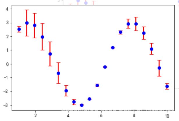
# plot the trend line with error bars that correspond to standard deviation  用与标准偏差相对应的误差线绘制趋势线
accuracies_mean = np.array([np.mean(v) for k,v in sorted(k_to_accuracies.items())])
accuracies_std = np.array([np.std(v) for k,v in sorted(k_to_accuracies.items())])
plt.errorbar(k_choices, accuracies_mean, yerr=accuracies_std)
plt.title('Cross-validation on k')
plt.xlabel('k')
plt.ylabel('Cross-validation accuracy')
plt.show()

1. plt.scatter绘制散点图

2. [k] * len(accuracies)就是将[k]复制len(accuracies)份，变成[k,k,k,k,k]。这里不是数值扩大len倍，而是复制多少份。

3. for k,v in sorted(k_to_accuracies.items())是访问一个排序好的字典迭代器，k得到键，v得到值，也就是一个列表，np.mean(v)计算平均值，np.std(v)计算标准差。这里可以看到，可以使用numpy计算列表的平均值

4. plt.errorbar函数解释

   plt.errorbar()函数解析（最清晰的解释）

   x,y: 数据点的位置坐标

   xerr,yerr: 数据的误差范围

   如下图所示，能看到y轴数据的大小，以及误差的范围，也就是标准差。

4.作业中的inline-questions深入理解（未必正确）

参考1：CS231n 2018作业1-KNN

参考2：

4.1.Inline Question 1

Notice the structured patterns in the distance matrix, where some rows or columns are visible brighter. (Note that with the default color scheme black indicates low distances while white indicates high distances.)
注意距离矩阵中的结构化图案，其中某些行或列的可见亮度更高。 （请注意，使用默认的配色方案，黑色表示低距离，而白色表示高距离。）

• What in the data is the cause behind the distinctly bright rows?

• What causes the columns?

  数据中哪些是明显亮行背后的原因？
  是什么原因造成了列？

$\text{Y}ourAnswer:$

• 1.行高亮：对于测试集中的当前行所处的图片，在训练集中所有的图片都与其不太相似，距离较远。意味着这张图片在训练集中找不到与其比较小相似的图片，说明这张图片噪声比较大，可能是错误的数据。
• 2.列高亮：训练集中当前列所处的图片，与测试集中的所有图片都不太相似。说明训练集的这张图片不具有代表性。

4.2.Inline Question 2

We can also use other distance metrics such as L1 distance.
For pixel values $p_{ij}^{(k)}$ at location $(i,j)$ of some image $I_k$,

the mean $\mu$ across all pixels over all images is $$\mu =\frac{1}{nhw}\sum _{k=1}^n\sum _{i=1}^h\sum _{j=1}^w{p}_{ij}^{(k)}$$
And the pixel-wise mean ${\mu }_{ij}$ across all images is
$${\mu }_{ij}=\frac{1}{n}\sum _{k=1}^n{p}_{ij}^{(k)}.$$
The general standard deviation $\sigma$ and pixel-wise standard deviation ${\sigma }_{ij}$ is defined similarly.

Which of the following preprocessing steps will not change the performance of a Nearest Neighbor classifier that uses L1 distance? Select all that apply.

1. Subtracting the mean $\mu$ (${\tilde{p}}_{ij}^{(k)}=p_{ij}^{(k)}-\mu$.)
2. Subtracting the per pixel mean ${\mu }_{ij}$ (${\tilde{p}}_{ij}^{(k)}=p_{ij}^{(k)}-{\mu }_{ij}$.)
3. Subtracting the mean $\mu$ and dividing by the standard deviation $\sigma$.
4. Subtracting the pixel-wise mean ${\mu }_{ij}$ and dividing by the pixel-wise standard deviation ${\sigma }_{ij}$.
5. Rotating the coordinate axes of the data.

$\text{Y}ourAnswer:$

• 1.2.3.4.5

$\text{Y}ourExplanation:$

• 1.对每张图片的所有像素都减去同一个值，L1距离显然不变
• 2.对每张图片的每个像素都减去同一个值，但是不同的像素点减去的值不一样，最后每个像素点的L1距离还是不变，总的L1距离也不变
• 3.对每张图片的所有像素减去同一个值，再除以标准差。乘除法会影响L1距离，但是并不影响L1距离的排序，故也不影响KNN的结果
• 4.解释同3
• 5.图片旋转后像素的对应位置不变，因此L1距离不变**？？？**不太理解这里旋转的意思

注意理解上面的定义：$\mu$是所有图片的所有像素的均值，${\mu }_{ij}$是所有图片在$(i,j)$像素点处的均值。方差的定义同理

4.3.Inline Question 3

Which of the following statements about $k$-Nearest Neighbor ($k$-NN) are true in a classification setting, and for all $k$? Select all that apply.

1. The decision boundary of the k-NN classifier is linear.
2. The training error of a 1-NN will always be lower than or equal to that of 5-NN.
3. The test error of a 1-NN will always be lower than that of a 5-NN.
4. The time needed to classify a test example with the k-NN classifier grows with the size of the training set.
5. None of the above.

$\text{Y}ourAnswer:$

2. 4

$\text{Y}ourExplanation:$

1. KNN不是线性的，看他的边界就知道，是由很多折线构成，也就是说它是局部线性的。
2. 这里的训练误差可以理解成将训练集记录下来之后，再拿出来部分训练集进行预测，得到的误差就是训练误差。很明显，此时每张测试图片都能在训练集中找到与其完全相同的，所以1-NN的训练误差是0。而5-NN的误差可能是0，比如5张图片分类都是相同的，要或大于0
3. 测试集误差1-NN总比5-NN小，很明显不对。测试集看的是数据的泛化能力。从前面的测试也能看出来，K属于超参数，需要调优，无法理论分析出哪个K最好
4. 数据量变大，显然。

5.注意事项

5.1.变量命令不要重复

在jupyter notebook中，每个cell中的变量都是通用的。比如从前到后的三个cell的顺序分别是A,B,C，A的cell中已经定义的变量，如果在B的cell中再次定义，会认为是赋值，这在无形中就增加了危险。因为如果后面C的cell打算用的是A的cell中的该变量，但是这个变量已经无意中由于重复定义导致值被更改了，就会出问题。

我就遇到了这个问题，在交叉评估中，我把验证集的个数还是定义成了num_test（其实是我从前面的cell中复制过来忘了改），实际应该定义成num_val，正常的话他们的值分别是num_test=500和num_val1000。这就导致最后我找到best_k测试准确率的时候只有14%左右，而正常在28%左右。