scikit-learn(sklearn)学习笔记十 支持向量机

书接上次笔记，我们通过把二维的数据映射到三维，再用超平面进行划分。但是这也是有很大的问题的，维数越高越难以计算。于是在上次笔记的最后，采用了更换核函数来满足支持向量机的分类要求。
klearn在skearn中可选择以下几种选项

• linear 线性核，解决问题为线性。
• poly 多项式核，解决问题为偏线性。
• sigmoid 双曲正切核，解决问题为非线性。
• rbf 高斯径向基，解决偏为非线性。
  所以要研究kernel应该如何选取

from sklearn.datasets import load_breast_cancer
from sklearn.svm import SVC
from sklearn.model_selection import train_test_split
import matplotlib.pyplot as plt
import numpy as np
from time import time
import datetime

data=load_breast_cancer()
X=data.data
y=data.target
#X.shape
#np.unique(y)
plt.scatter(X[:,0],X[:,1],c=y)
plt.show()

Xtrain,Xtest,Ytrain,Ytest=train_test_split(X,y,test_size=0.3,random_state=420)
Kernel=["linear","poly","rbf","sigmoid"]
for kernel in Kernel:
	time0=time()
	clf=SVC(kernel=kernel,gamma="auto",cache_size=5000).fit(Xtrain,Ytrain)
	print(kernel,clf.score(Xtest,Ytest))
	print(datetime.datetime.fromtimestamp(time()-time0).strftime("%M:%S:%f"))

linear 0.9298245614035088
00:00:505116

因为poly 多项式核还有一个参数degree默认的degree等于3，这让我电脑运行了很久都没有出结果，如果我把poly去掉。

linear 0.9298245614035088
00:00:487102
rbf 0.5964912280701754
00:00:053013
sigmoid 0.5964912280701754
00:00:005007

如果我将ploy中的degree改成等于三

linear 0.9298245614035088
00:00:491111
poly 0.9239766081871345
00:00:091014
rbf 0.5964912280701754
00:00:052018
sigmoid 0.5964912280701754
00:00:006002

那为什么看起来万能的rbf，他所提供模型的误差会比线性模型相差很多，我们先查看一下我们所用的数据集

data=pd.DataFrame(X)
data.describe([0.01,0.05,0.1,0.25,0.5,0.75,0.9,0.99]).T
    count        mean         std  ...          90%          99%         max
0   569.0   14.127292    3.524049  ...    19.530000    24.371600    28.11000
1   569.0   19.289649    4.301036  ...    24.992000    30.652000    39.28000
2   569.0   91.969033   24.298981  ...   129.100000   165.724000   188.50000
3   569.0  654.889104  351.914129  ...  1177.400000  1786.600000  2501.00000
4   569.0    0.096360    0.014064  ...     0.114820     0.132888     0.16340
5   569.0    0.104341    0.052813  ...     0.175460     0.277192     0.34540
6   569.0    0.088799    0.079720  ...     0.203040     0.351688     0.42680
7   569.0    0.048919    0.038803  ...     0.100420     0.164208     0.20120
8   569.0    0.181162    0.027414  ...     0.214940     0.259564     0.30400
9   569.0    0.062798    0.007060  ...     0.072266     0.085438     0.09744
10  569.0    0.405172    0.277313  ...     0.748880     1.291320     2.87300
11  569.0    1.216853    0.551648  ...     1.909400     2.915440     4.88500
12  569.0    2.866059    2.021855  ...     5.123200     9.690040    21.98000
13  569.0   40.337079   45.491006  ...    91.314000   177.684000   542.20000
14  569.0    0.007041    0.003003  ...     0.010410     0.017258     0.03113
15  569.0    0.025478    0.017908  ...     0.047602     0.089872     0.13540
16  569.0    0.031894    0.030186  ...     0.058520     0.122292     0.39600
17  569.0    0.011796    0.006170  ...     0.018688     0.031194     0.05279
18  569.0    0.020542    0.008266  ...     0.030120     0.052208     0.07895
19  569.0    0.003795    0.002646  ...     0.006185     0.012650     0.02984
20  569.0   16.269190    4.833242  ...    23.682000    30.762800    36.04000
21  569.0   25.677223    6.146258  ...    33.646000    41.802400    49.54000
22  569.0  107.261213   33.602542  ...   157.740000   208.304000   251.20000
23  569.0  880.583128  569.356993  ...  1673.000000  2918.160000  4254.00000
24  569.0    0.132369    0.022832  ...     0.161480     0.188908     0.22260
25  569.0    0.254265    0.157336  ...     0.447840     0.778644     1.05800
26  569.0    0.272188    0.208624  ...     0.571320     0.902380     1.25200
27  569.0    0.114606    0.065732  ...     0.208940     0.269216     0.29100
28  569.0    0.290076    0.061867  ...     0.360080     0.486908     0.66380
29  569.0    0.083946    0.018061  ...     0.106320     0.140628     0.20750

[30 rows x 13 columns]

通过观察平均值和方差，我们有理由怀疑量纲不是同一，数据的分布是偏态的，所以我们进行一下数据的标准化。

from sklearn.preprocessing import StandardScaler
X=StandardScaler().fit_transform(X)

我们再用这个数据集进行运算

linear 0.9766081871345029
00:00:008999
poly 0.9649122807017544
00:00:004002
rbf 0.9707602339181286
00:00:008001
sigmoid 0.9532163742690059
00:00:004001

我们可以发现线性核函数和高斯核函数的效果都十分的好，我们应该作何选择呢，线性核函数是没有参数的没有可以进行调整，而高斯核函数有gamma值可以调整，所以我们来画高斯核函数的学习曲线。

score=[]
gamma_range=np.logspace(-10,1,50)
for i in gamma_range:
	clf=SVC(kernel="rbf",gamma=i,cache_size=5000).fit(Xtrain,Ytrain)
	score.append(clf.score(Xtest,Ytest))
print(max(score),gamma_range[score.index(max(score))])
plt.plot(gamma_range,score)
plt.show()


0.9766081871345029 0.012067926406393264

我们一直假设训练样本在样本空间或特征空间食线性可分的，即存在一个超平面能将不同类的样本完全划分开。然而，在现实任务中往往很难确定合适的核函数使得训练样本在特征空间中线性可分；退一步说，即便恰好找到了某个核函数使训练样本在特征空间中线性可分，也很难断定这个貌似线性可分的结果不是由于过拟合造成的。缓解该问题的一个方法是允许支持向量机在一些样本上出错，为此要引入“软间隔”的概念。

score=[]
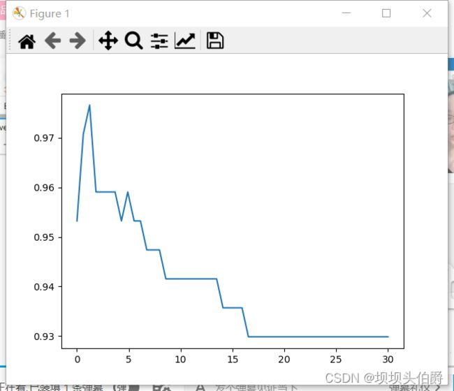
C_range=np.linspace(0.01,30,50)
for i in C_range:
	clf=SVC(kernel="linear",C=i,cache_size=5000).fit(Xtrain,Ytrain)
	score.append(clf.score(Xtest,Ytest))
print(max(score),C_range[score.index(max(score))])
plt.plot(C_range,score)
plt.show()

0.9766081871345029 1.2340816326530613

score=[]
C_range=np.linspace(0.01,30,50)
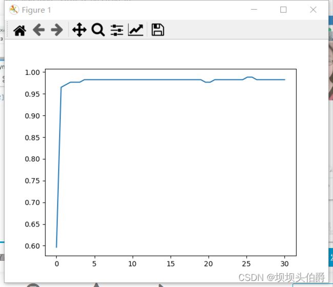
for i in C_range:
	clf=SVC(kernel="rbf",C=i,cache_size=5000).fit(Xtrain,Ytrain)
	score.append(clf.score(Xtest,Ytest))
print(max(score),C_range[score.index(max(score))])
plt.plot(C_range,score)
plt.show()

0.9883040935672515 25.103673469387758