机器学习——基于R的svm练习
步骤
- 1. 数据预处理
- 2. 建模
-
- 1. linear
- 2. polynomial
- 3. radial basis
- 4. sigmoid
- 3. 模型选择
- 4. 特征选择
- 5. 完整代码
本文参考:《精通机器学习:基于R》5.3节
数据集来自R包(MASS),包含了532位女性的信息,存储在两个数据框中,具体变量表述如下:
npreg:怀孕次数
glu:血糖浓度, 由口服葡萄糖耐量测试给出
bp:舒张压
skin:三头肌皮褶厚度
bmi:身体质量指数
ped:糖尿病家族影响因素
age:年龄
type:是否患有糖尿病(yes/no)
目的:研究这类人群,对可能导致糖尿病的风险因素进行预测。
1. 数据预处理
# 载入相关R包和数据
library(e1071)
library(caret)
library(MASS)
library(reshape2)
library(ggplot2)
library(kernlab)
# train
data("Pima.tr")
# test
data("Pima.te")
# 合并数据,便于把数据的特征可视化
pima <- rbind(Pima.tr, Pima.te)
pima.melt <- melt(pima, id.vars = "type")
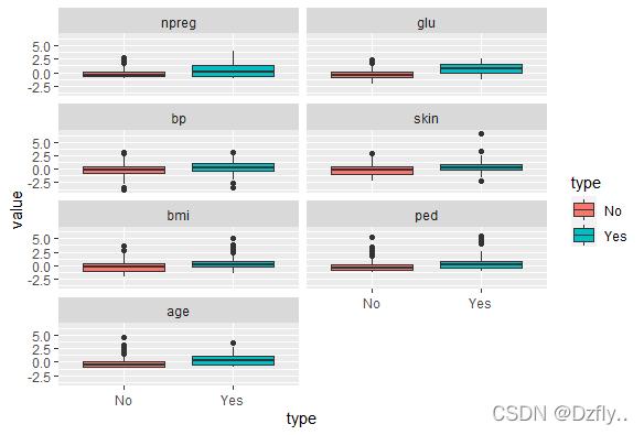
# 画箱线图进行对比
ggplot(data = pima.melt, aes(x = type, y = value, fill = type)) + geom_boxplot() +
facet_wrap(~ variable, ncol = 2)
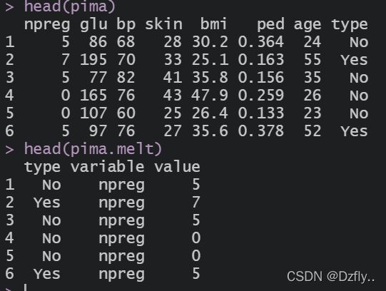

从图中可以看出,两种人群除了glu有明显的差距外,其余的都看不出来区别,原因就是这几种特征的数值差别太大,所以我们要对数据进行归一化处理,好让我们看到更明显的结果。
# data.frame格式的数据scale之后会自动变成一个矩阵,所以要重新将其变为data.frame
pima.scale <- data.frame(scale(pima[, -8]))
pima.scale$type <- pima$type
pima.scale.melt <- melt(pima.scale, id.vars = "type")
ggplot(data = pima.scale.melt, aes(x = type, y = value, fill = type)) + geom_boxplot() +
  facet_wrap(~ variable, ncol = 2)
这样作出的图就明显一些, 但其实只是从扁的变长了一点,还需要进一步分析。
> # 查看相关性
> cor(pima.scale[-8])
            npreg       glu          bp       skin         bmi         ped        age
npreg 1.000000000 0.1253296 0.204663421 0.09508511 0.008576282 0.007435104 0.64074687
glu   0.125329647 1.0000000 0.219177950 0.22659042 0.247079294 0.165817411 0.27890711
bp    0.204663421 0.2191779 1.000000000 0.22607244 0.307356904 0.008047249 0.34693872
skin  0.095085114 0.2265904 0.226072440 1.00000000 0.647422386 0.118635569 0.16133614
bmi   0.008576282 0.2470793 0.307356904 0.64742239 1.000000000 0.151107136 0.07343826
ped   0.007435104 0.1658174 0.008047249 0.11863557 0.151107136 1.000000000 0.07165413
age   0.640746866 0.2789071 0.346938723 0.16133614 0.073438257 0.071654133 1.00000000
可以看出,skin和bmi、npreg和age之间具有很高的相关性。但貌似还是看不出与type有多大关系,我们继续。
# 设置一个随机数种子,之后可以复现结果
set.seed(123)
# 把数据呼啦呼啦(随机打乱),然后三七分,七为训练集,三为测试集
ind <- sample(2, nrow(pima.scale), replace = TRUE, prob = c(0.7, 0.3))
train <- pima.scale[ind == 1, ]
test <- pima.scale[ind == 2, ]
2. 建模
我们使用e1071包来构建svm模型,e1071包中的svm()包含四种内核,我们依次测试四种kernel,看哪一个结果最好。不过在这里我们使用tune.svm(),因为该函数可以进行参数调优,kernel的种类也是可以选择的。
kernel
the kernel used in training and predicting. You might consider changing some of the following parameters, depending on the kernel type.linear:
*u’v
polynomial:
(gamma*u’v + coef0)^degree
radial basis:
exp(-gamma|u-v|^2)
sigmoid:
*tanh(gamma*u’v + coef0)
1. linear
# linear
set.seed(123)
# 寻找最优参数
linear.tune <- tune.svm(type ~., data = train, kernal = "linear",
                        cost = c(0.001, 0.01, 0.1, 1, 5, 10))
summary(linear.tune)

# 利用最优模型来预测
best.linear <- linear.tune$best.model
linear.test <- predict(best.linear, newdata = test)

# 查看预测准确率
linear.tab <- table(linear.test, test$type)
linear.tab
# diag():对角线相加
sum(diag(linear.tab))/sum(linear.tab)

可以看到当cost=1时,模型是最优的。此时的预测准确率约为77.5%。(结果与书本上略有不同,是因为数据集随即划分时,设置的种子不同)
其实在寻找最优参数时,我们无法知道具体的数值,所以可以设置一个数组,然后逐个去试,如下
# cost初始值为0.1,每次增加0.1,最大到5
linear.tune <- tune.svm(type ~., data = train, kernal = "linear",
                        cost = seq(0.1, 5, 0.1))
summary(linear.tune)
best.linear <- linear.tune$best.model
linear.test <- predict(best.linear, newdata = test)
linear.tab <- table(linear.test, test$type)
linear.tab
sum(diag(linear.tab))/sum(linear.tab)

#########################################
> linear.tab
linear.test No Yes
        No  87  23
        Yes 12  29
> sum(diag(linear.tab))/sum(linear.tab)
[1] 0.7682119
#########################################

可以看到,cost的取值略有不同,且误分类误差率也降低了一点点。但是!!!但是准确率也并没有提高,而是下降了一点点。
2. polynomial
# polynomial
set.seed(123)
poly.tune <- tune.svm(type ~ ., data = train, kernel = "polynomial",
                      degree = c(3, 4, 5), coef0 = c(0.1, 0.5, 1, 2, 3, 4))
summary(poly.tune)
best.poly <- poly.tune$best.model
poly.test <- predict(best.poly, newdata = test)
poly.tab <- table(poly.test, test$type)
poly.tab
sum(diag(poly.tab))/sum(poly.tab)


####################################
> poly.tab
poly.test No Yes
      No  88  26
      Yes 11  26
> sum(diag(poly.tab))/sum(poly.tab)
[1] 0.7549669
####################################

准确率约为75.5%,不如linear。同理也可以进行参数逐步优化。
poly.tune <- tune.svm(type ~ ., data = train, kernel = "polynomial",
                      degree = seq(2, 4, 0.1), coef0 = seq(0, 0.5, 0.1))
summary(poly.tune)
best.poly <- poly.tune$best.model
poly.test <- predict(best.poly, newdata = test)
poly.tab <- table(poly.test, test$type)
poly.tab
sum(diag(poly.tab))/sum(poly.tab)


################################################
> summary(poly.tune)

Parameter tuning of ‘svm’:

- sampling method: 10-fold cross validation

- best parameters:
 degree coef0
      2   0.1

- best performance: 0.2148448

> poly.tab

poly.test No Yes
      No  87  23
      Yes 12  29

> sum(diag(poly.tab))/sum(poly.tab)
[1] 0.7682119
################################################
这里degree的最优值由3变成了2,coef0没有变化,且最终的准确率是有提升的,约为76.8%,但不如linear。
3. radial basis
# radial basis
set.seed(123)
rbf.tune <- tune.svm(type ~., data = train, kernal = "radial",
                        gamma = c(0.1, 0.5, 1, 2, 3, 4))
summary(rbf.tune)
best.rbf <- rbf.tune$best.model
rbf.test <- predict(best.rbf, newdata = test)
rbf.tab <- table(rbf.test, test$type)
rbf.tab
sum(diag(rbf.tab))/sum(rbf.tab)

准确率约为76.8%,差别不大。
4. sigmoid
# sigmoid
set.seed(123)
sigmod.tune <- tune.svm(type ~., data = train, kernal = "sigmoid",
                     gamma = c(0.1, 0.5, 1, 2, 3, 4),
                     coef0 = 2)
summary(sigmod.tune)
best.sigmod <- sigmod.tune$best.model
sigmod.test <- predict(best.sigmod, newdata = test)
sigmod.tab <- table(sigmod.test, test$type)
sigmod.tab
sum(diag(sigmod.tab))/sum(sigmod.tab)


##########################################
> sigmod.tab

sigmod.test No Yes
        No  87  23
        Yes 12  29
> sum(diag(sigmod.tab))/sum(sigmod.tab)
[1] 0.7682119
##########################################

可以看出,四种kernel的准确率其实都比较接近,想要明显提高准确率,还需要进行其他优化。
3. 模型选择
# sigmod 与 linear 模型比较
confusionMatrix(sigmod.test, test$type, positive = "Yes")

############################################
Confusion Matrix and Statistics

          Reference
Prediction No Yes
       No  87  23
       Yes 12  29

               Accuracy : 0.7682
                 95% CI : (0.6927, 0.8329)
    No Information Rate : 0.6556
    P-Value [Acc > NIR] : 0.001831

                  Kappa : 0.4596

 Mcnemar s Test P-Value : 0.090969

            Sensitivity : 0.5577
            Specificity : 0.8788
         Pos Pred Value : 0.7073
         Neg Pred Value : 0.7909
             Prevalence : 0.3444
         Detection Rate : 0.1921
   Detection Prevalence : 0.2715
      Balanced Accuracy : 0.7182

       'Positive' Class : Yes
############################################


confusionMatrix(linear.test, test$type, positive = "Yes")

############################################
Confusion Matrix and Statistics

          Reference
Prediction No Yes
       No  88  23
       Yes 11  29

               Accuracy : 0.7748
                 95% CI : (0.6998, 0.8387)
    No Information Rate : 0.6556
    P-Value [Acc > NIR] : 0.001001

                  Kappa : 0.4725

 Mcnemar s Test P-Value : 0.059230

            Sensitivity : 0.5577
            Specificity : 0.8889
         Pos Pred Value : 0.7250
         Neg Pred Value : 0.7928
             Prevalence : 0.3444
         Detection Rate : 0.1921
   Detection Prevalence : 0.2649
      Balanced Accuracy : 0.7233

       'Positive' Class : Yes
############################################
这个结果只能说难分伯仲。在这里,我们只是把特征堆叠在一起,作为所谓的输入空间,然后让SVM这个黑盒去计算,最后给出一个预测分类。所以想要提高预测准确率,还需要从多方面入手。
4. 特征选择
# 粗略的特征选择
set.seed(123)
rfeCNTL <- rfeControl(functions = lrFuncs, method = "cv", number = 10)
svm.feature <- rfe(train[, 1:7], train[, 8], sizes = c(7, 6, 5, 4),
                   rfeControl = rfeCNTL, method = "svmLinear")
svm.feature

#################################################################
Recursive feature selection

Outer resampling method: Cross-Validated (10 fold)

Resampling performance over subset size:

 Variables Accuracy  Kappa AccuracySD KappaSD Selected
         4   0.7751 0.4652    0.06046  0.1381
         5   0.7802 0.4758    0.05477  0.1297
         6   0.7853 0.4872    0.05300  0.1218
         7   0.7880 0.4894    0.05222  0.1345        *

The top 5 variables (out of 7):
   glu, bmi, ped, age, npreg
#################################################################

svm.5 <- svm(type ~ glu + bmi + ped + age + npreg, data = train,
             kernel = "linear")
svm.5.predict <- predict(svm.5, newdata = test[c(1, 2, 5, 6, 7)])
svm.5.tab <- table(svm.5.predict, test$type)
svm.5.tab
sum(diag(svm.5.tab))/sum(svm.5.tab)

#################################################################
> svm.5.tab

svm.5.predict No Yes
          No  86  18
          Yes 13  34
> sum(diag(svm.5.tab))/sum(svm.5.tab)
[1] 0.794702
#################################################################
粗略的特征选择表示,五特征模型表现得比较好,五个特征分别为:glu, bmi, ped, age, npreg。用五特征模型进行预测的准确率竟然是最高的79.4%。虽然也没高多少,但是说明特征选择还是有用滴。
5. 完整代码
library(e1071)
library(caret)
library(MASS)
library(reshape2)
library(ggplot2)
library(kernlab)

data("Pima.tr")
data("Pima.te")

# 画箱线图进行对比
pima <- rbind(Pima.tr, Pima.te)
pima.melt <- melt(pima, id.vars = "type")
ggplot(data = pima.melt, aes(x = type, y = value, fill = type)) +
  geom_boxplot() + facet_wrap(~ variable, ncol = 2)

# 归一化
pima.scale <- data.frame(scale(pima[, -8]))
pima.scale$type <- pima$type
pima.scale.melt <- melt(pima.scale, id.vars = "type")
ggplot(data = pima.scale.melt, aes(x = type, y = value, fill = type)) +
  geom_boxplot() + facet_wrap(~ variable, ncol = 2)

# 查看相关性
cor(pima.scale[-8])

# 划分训练集与测试集
set.seed(123)
ind <- sample(2, nrow(pima.scale), replace = TRUE, prob = c(0.7, 0.3))
train <- pima.scale[ind == 1, ]
test <- pima.scale[ind == 2, ]

# SVM
# linear
set.seed(123)
linear.tune <- tune.svm(type ~., data = train, kernal = "linear",
                        cost = c(0.001, 0.01, 0.1, 1, 5, 10))
summary(linear.tune)
# linear.tune <- tune.svm(type ~., data = train, kernal = "linear",
#                         cost = seq(0.1, 5, 0.1))
# summary(linear.tune)
best.linear <- linear.tune$best.model
linear.test <- predict(best.linear, newdata = test)
linear.tab <- table(linear.test, test$type)
linear.tab
sum(diag(linear.tab))/sum(linear.tab)

# polynomial
set.seed(123)
poly.tune <- tune.svm(type ~ ., data = train, kernel = "polynomial",
                      degree = c(3, 4, 5), coef0 = c(0.1, 0.5, 1, 2, 3, 4))
summary(poly.tune)
# poly.tune <- tune.svm(type ~ ., data = train, kernel = "polynomial",
#                       degree = seq(2, 4, 0.1), coef0 = seq(0, 0.5, 0.1))
# summary(poly.tune)
best.poly <- poly.tune$best.model
poly.test <- predict(best.poly, newdata = test)
poly.tab <- table(poly.test, test$type)
poly.tab
sum(diag(poly.tab))/sum(poly.tab)

# radial basis
set.seed(123)
rbf.tune <- tune.svm(type ~., data = train, kernal = "radial",
                        gamma = c(0.1, 0.5, 1, 2, 3, 4))
summary(rbf.tune)
best.rbf <- rbf.tune$best.model
rbf.test <- predict(best.rbf, newdata = test)
rbf.tab <- table(rbf.test, test$type)
rbf.tab
sum(diag(rbf.tab))/sum(rbf.tab)

# sigmoid
set.seed(123)
sigmod.tune <- tune.svm(type ~., data = train, kernal = "sigmoid",
                     gamma = c(0.1, 0.5, 1, 2, 3, 4),
                     coef0 = c(0.1, 0.5, 1, 2, 3, 4))
summary(sigmod.tune)
best.sigmod <- sigmod.tune$best.model
sigmod.test <- predict(best.sigmod, newdata = test)
sigmod.tab <- table(sigmod.test, test$type)
sigmod.tab
sum(diag(sigmod.tab))/sum(sigmod.tab)

# 模型比较
confusionMatrix(sigmod.test, test$type, positive = "Yes")
confusionMatrix(linear.test, test$type, positive = "Yes")

# 粗略的特征选择
set.seed(123)
rfeCNTL <- rfeControl(functions = lrFuncs, method = "cv", number = 10)
svm.feature <- rfe(train[, 1:7], train[, 8], sizes = c(7, 6, 5, 4),
                   rfeControl = rfeCNTL, method = "svmLinear")
svm.feature

svm.5 <- svm(type ~ glu + bmi + ped + age + npreg, data = train,
             kernel = "linear")
svm.5.predict <- predict(svm.5, newdata = test[c(1, 2, 5, 6, 7)])
svm.5.tab <- table(svm.5.predict, test$type)
svm.5.tab
sum(diag(svm.5.tab))/sum(svm.5.tab)