拉普拉斯网格变形：Laplacian Mesh Deformation 附Python代码实现

本文介绍一种非常巧妙的网格变换方法：拉普拉斯变换。它最重要的一个好处是可以保局部特征不变。和多视角几何中的保角度、保平行、保交比（cross ratio）等变换一样非常重要。

1.动机

传统的基于笛卡尔坐标系的三维曲面表达方式，只能描述每个顶点的空间位置信息。而基于曲面微分表达的方式能够描述包括尺寸和方向在内的局部信息。拉普拉斯坐标蕴含着曲面的局部特征信息，网格曲面的拉普拉斯坐标其在网格变形、网格平滑、网格去噪等方面都用着重要的应用。因此本论文基于拉普拉斯算子进行介绍。推荐论文《Laplacian Mesh Optimization》

2.基本定义

我们让$\mathcal{M}=(V,E,F)$表示为一个三角网格，其中$V$为顶点，有$n$个。$E$表示顶点之间的边，$F$表示三角网格的面片（Face）。对于每一个属于$\mathcal{M}$的顶点${\text{v}}_i=(x_i,y_i,z_i)$，均为传统的笛卡尔坐标。

2.1 顶点${\text{v}}_i$的拉普拉斯
顶点${\text{v}}_i$的拉普拉斯或者顶点${\text{v}}_i的\delta$坐标的定义如下：
$${\delta }_i=({\delta }_i^x,{\delta }_i^y,{\delta }_i^z)={\text{v}}_i-\sum _{j\in N(i)}{w}_{ij}{\text{v}}_j\text{\hspace{1em}(1)}$$
其中$w_{ij}=\frac{{\omega }_{ij}}{{\sum }_{k\in N(i)}{\omega }_{ik}}$。由于${\sum }_{j\in N(i)}{w}_{ij}=1$，那么有${\text{v}}_i={\sum }_{j\in N(i)}{w}_{ij}{\text{v}}_i$。所以式子（1）可以写成：
$${\delta }_i=\sum _{j\in N(i)}{w}_{ij}({\text{v}}_i-{\text{v}}_j)\text{\hspace{1em}(2)}$$其中$N(i)=\left\{j|(i,j)\in E\right\}$表示为所有与顶点${\text{v}}_i$能够构成边的顶点，也就是领域顶点。而把顶点${\text{v}}_i\to {\delta }_i$转换的矩阵叫做拉普拉斯矩阵。对权值$w_{ij}$中的${\omega }_{ij}$选择有下面比较流行的两种：
$$\begin{gathered} {\omega }_{ij}=1 \\ {\omega }_{ij}=\cot {\alpha }_{ij}+\cot {\beta }_{ij}\text{\hspace{1em}(3)} \end{gathered}$$

首先吐槽一下，大部分中文博客一上来就用$d_i=\Vert N(i)\Vert$的情况来讲拉普拉斯矩阵，我觉得非常容易误导读者，先给出（2）式中的一般性结论，再来讨论各自特殊情况比较好。包括后面从$\delta$到$V$的重建，写的也是不知所云。

2.2 拉普拉斯矩阵
为了获得上述2.1中顶点$V$的拉普拉斯：$\delta$，我们使用一个$n\times n$的矩阵$L$，对顶点矩阵$V$进行左乘：
$${\delta }_{n\times 3}=L_{n\times n}{V}_{n\times 3}\text{\hspace{1em}(4)}$$
而拉普拉斯矩阵$L$的定义如下：
$$L_{ij}=\{\begin{array}{ll}1& i=j\\ -w_{ij}& (i,j)\in E\\ 0& 其它\end{array}\text{\hspace{1em}(5)}$$
这个公式不需要推导，对等式（2）转换成矩阵形式$\delta =LV$就可以得到。

2.3 均值拉普拉斯
当我们取${\omega }_{ij}=1$，即$w_{ij}=\frac{1}{{\sum }_{k\in N(i)}1}$，我们令${\sum }_{k\in N(i)}1=\Vert N(i)\Vert$，其中$\Vert N(i)\Vert$为邻域顶点的数量：
$${\delta }_i=\sum _{j\in N(i)}\frac{1}{\Vert N(i)\Vert }({\text{v}}_i-{\text{v}}_j)\text{\hspace{1em}(6)}$$

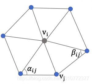
而这个式子明显就是向量$({\text{v}}_i-{\text{v}}_j)$的均值，于是它的方向代表局部$N(i)$的法向量方向，幅值代表平均曲率大小。这说明$\delta$坐标天然包含了形状的局部信息。一个可视化的例子如下图所示：

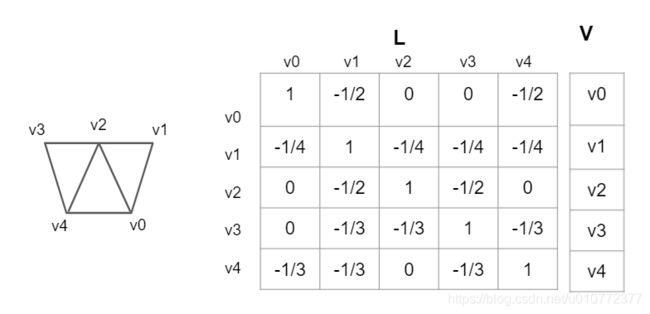
2.3.1 均值拉普拉斯矩阵$L$
为了形象化均值拉普拉斯矩阵，我用下图中的例子进行了可视化，结合公式（5）检查一下是不是这样：

2.4 余切拉普拉斯
为了获得网格更好的变形过程中逼近的性能，可以使用余切$\omega$代替均值$\omega$，余切$\omega$的定义如下：
$${\omega }_{ij}=\cot {\alpha }_{ij}+\cot {\beta }_{ij}\text{\hspace{1em}(7)}$$
那么权值$w_{ij}$:
$$w_{ij}=\frac{\cot {\alpha }_{ij}+\cot {\beta }_{ij}}{{\sum }_{k\in N(i)}\cot {\alpha }_{ik}+\cot {\beta }_{ik}}$$
其余切拉普拉斯为：
$${\delta }_i=\frac{1}{\Vert {\Omega }_i\Vert }\sum _{j\in N(i)}\cot {\alpha }_{ij}+\cot {\beta }_{ij}({\text{v}}_i-{\text{v}}_j)\text{\hspace{1em}(8)}$$
其中${\alpha }_{ij}$与${\beta }_{ij}$是如下图所示的两个角度，有时候也叫外角，但是这个外角和初中三角几何中的外角不一样，它们之间的和是180°。$\cot$ 为余切函数。

而权值项中的$\frac{1}{\Vert {\Omega }_i\Vert }$根据权值求和等于1的要求，很显然为：
$$\Vert {\Omega }_i\Vert =\sum _{k\in N(i)}\cot {\alpha }_{ik}+\cot {\beta }_{ik}\text{\hspace{1em}(9)}$$，
这个没有任何值得怀疑的。很多博客写着要计算voronoi region面积的，当然也可以，这其实就不是严格意义上的权重求和为1了。其实是对$\delta$进行了缩放，就是为了处理余切会出现负值以及在顶点非线性的问题。比如在论文《Laplacian Mesh Optimization》中就使用了$\Vert {\Omega }_i\Vert =4A({\text{v}}_i)$而：
$$\Vert {\Omega }_i\Vert =4A({\text{v}}_i)=\frac{1}{2}\sum _{k\in N(i)}(\cot {\alpha }_{ik}+\cot {\beta }_{ik})\ast \Vert {\text{v}}_i-{\text{v}}_k{\Vert }^2\text{\hspace{1em}(10)}$$

3. 拉普拉斯变换的应用

对于一个笛卡尔坐标的网格顶点$V$，假设它的拉普拉斯矩阵$L$我们已经给定，那么它的$\delta$坐标也就可以通过$\delta =LV$得到。如果到此为止，那么拉普拉斯变换:$LV\to \delta$也就是一个普通的线性变换，即如果$V\ne V^{{}^{\prime }}$，那么很可能导致$\delta \ne {\delta }^{{}^{\prime }}$。就像我们在做非刚体配准的时候，构造的方程$AX=b$中，矩阵$A$是满秩的，所以有唯一确定解，它不具备保局部结构的性质。

所以我们看一下，拉普拉斯变换是不是这种情况？关键是看矩阵$L$是不是满秩

我们把$LV=\delta$这个问题可以用下面的通用线性方程组表示：
$$AX=b\text{\hspace{1em}(11)}$$

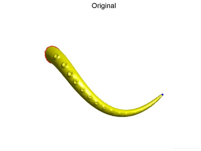
如果矩阵$A$是奇异矩阵，那么不同的$X$会有相同的$b$矩阵（因为对于奇异矩阵$A$，在给定$b$的情况下，有无数个$X^{{}^{\prime }}$满足$A{X}^{{}^{\prime }}=b$）。回到拉普拉斯变换，对于均值拉普拉斯矩阵$L$来说，是一个它的拓扑属性，在形变过程中不会改变。而我们在改变$V$的情况下，$\delta$有可能保持不变（注意这里是有可能）。这就意味着，我们在对网格顶点进行较大变动$V\to V^{{}^{\prime }}$的情况下，$V$和$V^{{}^{\prime }}$的局部结构$\delta$是保持不变的。这在动画领域非常重要。如下图所示的例子，对于一个章鱼的触须，我们希望它在改变笛卡尔坐标$V\to V^{{}^{\prime }}$的时候，它的局部结构，比如圆孔保持不变，这种形变才符合现实环境中的形变特征。这就是拉普拉斯形变的作用。

说了这么多，要回答上述问题，就要判断拉普拉斯矩阵$L$的秩是不是满秩

我们注意观察2.3.1章节中的图片中的$L$矩阵，如果对第一列加上其它剩余所有列（2-5列）那么，第一列就是$0$向量。因此很明显它的秩非满秩，不可逆。那么它的秩具体是多少呢？，原文作者给出了答案：
$$Rank(L)=n-k\text{\hspace{1em}(12)}$$
$k$为连通量的个数，在我们2.3.1例图的网格中，任何一个顶点都有通路到达任何一个其它顶点，它的连通数量就是1。因此它的秩就是4。

到目前为止，我们得到了满意的答案：拉普拉斯矩阵$L$，可以让$\delta$在顶点$V$改变的情况下，保持不变，即保局部结构不变。联想一下保角变换(conformal mapping)，保交比变换（投影变换的唯一保持不变的特征）。拉普拉斯变换就是保局部结构不变。

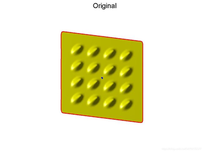
因此我们现在要做的就是怎么利用拉普拉斯变换的保局部结构不变?很显然我们需要在这个过程中，如前所述对于网格自身拓扑属性$L$一直是不变的，同时$\delta$也保持不变（这样才能保局部不变）。在$L$，$\delta$不变的情况下，我们需要知道经过形变后的卡迪尔坐标$V^{{}^{\prime }}$。作者提出的方法是给方程（11）加锚点，即在矩阵$L$和矩阵$\delta$中分别加上已知点。加锚点也是获得网格笛卡尔坐标系下形变:$V\to V^{{}^{\prime }}$的唯一来源，即如果不加锚点，网格就不变形（因为它的解有无穷个，$V$不知道往哪里进行变形。）。如下图所示，对于原始网格，只要以蓝色的点为锚点，把它进行拉扯，就能获得原始网格新的位置，并且在这个过程中局部结构保持不变。

$$\left[\begin{array}{c}{L}_{}\\ L_{anchor}\end{array}\right]V=\left[\begin{array}{c}\delta \\ {\delta }_{anchor}\end{array}\right]\text{\hspace{1em}(13)}$$

锚点添加
添加$m$个锚点的公式如下：
$$\left(\begin{array}{c}{L}_{n\times n}\\ L_{m\times n}^{anchor}\end{array}\right)V=\left(\begin{array}{c}{\delta }_{n\times 3}\\ {\delta }_{m\times 3}^{anchor}\end{array}\right)\text{\hspace{1em}(13)}$$
为了更容易理解，以我们在2.3.1中的例子为例。在拉普拉斯矩阵$L$中加锚点就是如果以第一个1个顶点为锚点，那么它的第一列的值为1，其它为0。同时指出第一个顶点，经过拉扯后的坐标：${\delta }_{anchor1}$，这个坐标是笛卡尔坐标，不是$\delta$坐标系下的坐标。即${\delta }_{anchor1}$,${\delta }_{anchor2}$是原始网格顶点v0, v3，将要形变到新位置的笛卡尔坐标。注意，我们经常需要对$L_{m\times n}^{anchor}$和${\delta }_{m\times 3}^{anchor}$中每个元素乘以一个统一的权重系数进行调整，不然形变后会出现对锚点过度拟合，而局部特征丢失的问题。

加锚点之后，如式子（13）就成了一个超定的方程组（方程个数大于未知量个数），有唯一最小二乘解。很显然可以通过下面的式子求解：
$$V={\left({\left(\begin{array}{c}{L}_{n\times n}\\ L_{m\times n}^{anchor}\end{array}\right)}^T\left(\begin{array}{c}{L}_{n\times n}\\ L_{m\times n}^{anchor}\end{array}\right)\right)}^{-1}{\left(\begin{array}{c}{L}_{n\times n}\\ L_{m\times n}^{anchor}\end{array}\right)}^T\left(\begin{array}{c}{\delta }_{n\times 3}\\ {\delta }_{m\times 3}^{anchor}\end{array}\right)$$

加锚点的时候，通常我们一个完整的网格，连通量为1。那么至少需要一个锚点。在实际过程中，为了获得更多形变控制，我们可以设置多个锚点（固定锚点、移动锚点）来更好获得我们想要的形变结果。因为对方程的约束点越多，越容易获得我们想要的结果。如下所示例子，不仅有$\mathcal{F}$处的固定锚点，还有$\mathcal{H}$处的移动锚点。如果没有固定锚点，那不能保证形变结果如右图所示

4. 代码实现

class LapMeshDeform():
    def __init__(self, verts, faces):
        self.verts = verts # numpy array with shape of [n_v, 3], n_v is the number of  vertices
        self.faces = faces # numpy array with shape of [n_f, 3], n_f is the number of vertices
    
    def _compute_edge(self):
        '''
        given faces with numpy array of [n_f, 3], return its edges[num_edge, 2], in addition edges[:, 0] < edges[:, 1].
        we do this sorting operation in edges' array for removing duplicated elements.
        For example self.faces[[0, 1, 2],
                               [0, 3, 1],
                               [0, 2, 4],
                              ]
        The returned edges will be: [[0, 1],
                                     [0, 2],
                                     [0, 3],
                                     [0, 4],
                                     [1, 2],
                                     [1, 3],
                                     [2, 4],
                                    ]
        
        Args:
            self.faces: numpy array with size of [n_f, 3], n_f is the number of faces.
        
        Return:
            uni_all_edge: numpy array with size of [n_e, 2], n_e is the number of edges.
            
        '''
        # get the edges of triangles. numpy array with shape [n_f, 2]
        edge_v0v1 = self.faces[:, [0, 1]] # edge of v0---v1
        edge_v0v2 = self.faces[:, [0, 2]] # edge of v0---v2
        edge_v1v2 = self.faces[:, [1, 2]] # edge of v1---v2

        # sorting the vertex index in edges for the purpose of removing duplicated elements.
        # for example if edge_v0v1[i, :] = [4, 1]. we will change edge_v0v1[i, :] to be [1, 4]
        edge_v0v1.sort()
        edge_v0v2.sort()
        edge_v1v2.sort()

        all_edge = np.vstack((edge_v0v1, edge_v0v2, edge_v1v2)) # numpy array with shape [n_f*3, 2]
        
        # remove duplicated edges
        uni_all_edge = np.unique(all_edge, axis=0)

        return uni_all_edge

    
    def uniform_laplacian(self):
        '''
        computing the uniform laplacian matrix L, L is an n by n matrix sparse matrix. 
        See the reference of <>
                   --  =   1 ,       if i=j   
        L[i, j] --|    =  -wij,      wij = 1/|N(i)|if (i, j) belong to an edge of a face
                   --  =   0       , others.
        
        Args:
            self.faces: numpy array with shape of [n_f, 3], mesh's faces.
            self.verts: numpy array with shape of [n_v, 3], mesh's vertices.
                        we only used its n_v to create [n_v, n_v] sparse matrix.
        
        Return:
            lap_matrix: the returned Laplacian matrix, it is a spare matrix.

        '''
        # initial the laplacian matrix(i.e. L) of self.faces. with the shape of [n_v, n_v], n_v is the number of vertices
        lap_matrix = sparse.lil_matrix((self.verts.shape[0], self.verts.shape[0]), dtype=np.float32)
        
        # get the edges with sorted index. the edges_sorted is with the shape of [n_e, 2]
        edges_sorted = self._compute_edge()
        lap_matrix[edges_sorted[:, 0], edges_sorted[:, 1]] = 1 # L[i, j] = 1, for edge i----j 
        lap_matrix[edges_sorted[:, 1], edges_sorted[:, 0]] = 1 # L[j, i] = 1, for edge i----j
        lap_matrix = normalize(lap_matrix, norm='l1', axis=1)*-1  # normaliz the L[i, j], for edge i----j . to -1/|N(i)|

        unit_diagonal = identity(self.verts.shape[0], dtype=np.float32) # L[i,j] = 1, if i=j
        lap_matrix += unit_diagonal

        return lap_matrix

        

    def cot_laplacian(self, area_normalize=True):
        '''
        computing the uniform laplacian matrix L, L is an n by n matrix sparse matrix. 
        See the reference of <> for definition of the cot weight.
                   --  =   1 ,       if i=j   
        L[i, j] --|    =  -wij,    wij = (cotαij + cotβij)/4A(i). 4A(i) = 0.5*sum_(k in N(i)) (cotαkj + cotβkj)|vi-vk|^2  
                   --  =   0       , others.
        
        This operation of cot_laplacian use the area normalize. It's sum of weight not equal to 1.
        To compute the size of Voronoi regions : A(i)
        I follow the reference https://stackoverflow.com/questions/13882225/compute-the-size-of-voronoi-regions-from-delaunay-triangulation
        The cotαik*|vi-vk| = H, H is the length of perpendicular line from vertices of αik to edge vi---vk.
        so 0.5*cotαik*|vi-vk|^2 is the area of triangle which contain edge of vi---vk, and angle of αkj.

        Args:
            self.faces: numpy array with shape of [n_f, 3], mesh's faces.
            self.verts: numpy array with shape of [n_v, 3], mesh's vertices.
                        we only used its n_v to create [n_v, n_v] sparse matrix.
            area_normalize: True for wij = (cotαij + cotβij)/4A(i) depicted above.
                            False for wij = (cotαij + cotβij)/sum_(k in N(i)) (cotαkj + cotβkj)
        
        Return:
            lap_matrix: the returned Laplacian matrix, it is a spare matrix.
        '''
        # initial the laplacian matrix(i.e. L) of self.faces. with the shape of [n_v, n_v], n_v is the number of vertices
        lap_matrix = sparse.lil_matrix((self.verts.shape[0], self.verts.shape[0]), dtype=np.float32)
        sum_area_vert = np.zeros([self.verts.shape[0], 1])

        # get the vertex index of edges of triangles. numpy array with shape [n_f, 2].
        edge_v0v1 = self.faces[:, [0, 1]]  # edge of v0---v1
        edge_v0v2 = self.faces[:, [0, 2]]  # edge of v0---v2
        edge_v1v2 = self.faces[:, [1, 2]]  # edge of v1---v2

        # compute length of edges, numpy array, shape is (n_f, )
        length_edge_v0v1 = np.linalg.norm(self.verts[edge_v0v1[:, 0], :]-self.verts[edge_v0v1[:, 1], :], axis=1)
        length_edge_v0v2 = np.linalg.norm(self.verts[edge_v0v2[:, 0], :]-self.verts[edge_v0v2[:, 1], :], axis=1)
        length_edge_v1v2 = np.linalg.norm(self.verts[edge_v1v2[:, 0], :]-self.verts[edge_v1v2[:, 1], :], axis=1)

        # compute area of each triangle see the reference https://pythonguides.com/find-area-of-a-triangle-in-python/
        # faces_area is numpy array with shape: (n_f, )
        average_edge_len = (length_edge_v0v1+ length_edge_v0v2 + length_edge_v1v2)/2.0
        faces_area = (average_edge_len*(average_edge_len- length_edge_v0v1)*(average_edge_len- length_edge_v0v2)*(average_edge_len- length_edge_v1v2))**0.5
        
        # compute the cot value of angle, the angle is face towards to edges.
        # cot value is numpy array with shape of (n_f, )
        cot_value_angle_face_v0v1 = (length_edge_v1v2**2 + length_edge_v0v2**2 - length_edge_v0v1**2)/(4*faces_area)
        cot_value_angle_face_v0v2 = (length_edge_v1v2**2 + length_edge_v0v1**2 - length_edge_v0v2**2)/(4*faces_area)
        cot_value_angle_face_v1v2 = (length_edge_v0v2**2 + length_edge_v0v1**2 - length_edge_v1v2**2)/(4*faces_area)

        # sum the triangles' area of vertices belong to.
        # the sum_area_vert is numpy array, shape is (n_v, 1)
        for i in range(faces_area.shape[0]):
            sum_area_vert[self.faces[i, 0]] += faces_area[i]
            sum_area_vert[self.faces[i, 1]] += faces_area[i]
            sum_area_vert[self.faces[i, 2]] += faces_area[i]
        
        
        # cot laplacian matrix
        for j in range(edge_v0v1.shape[0]):
            lap_matrix[edge_v0v1[j, 0], edge_v0v1[j, 1]] += cot_value_angle_face_v0v1[j]
            lap_matrix[edge_v0v1[j, 1], edge_v0v1[j, 0]] += cot_value_angle_face_v0v1[j]
            lap_matrix[edge_v0v2[j, 0], edge_v0v2[j, 1]] += cot_value_angle_face_v0v2[j]
            lap_matrix[edge_v0v2[j, 1], edge_v0v2[j, 0]] += cot_value_angle_face_v0v2[j]
            lap_matrix[edge_v1v2[j, 0], edge_v1v2[j, 1]] += cot_value_angle_face_v1v2[j]
            lap_matrix[edge_v1v2[j, 1], edge_v1v2[j, 0]] += cot_value_angle_face_v1v2[j]
        
        lap_matrix_nonormalize = lap_matrix.copy()
        if area_normalize:
            # normalize wij with the size of Voronoi regions: 4A(i) = 0.5*sum_(k in N(i)) (cotαkj + cotβkj)|vi-vk|^2  
            for k in range(self.verts.shape[0]):
                if sum_area_vert[k, :] != 0:
                    lap_matrix[k, :] = lap_matrix[k, :]/(sum_area_vert[k, :])
            lap_matrix = lap_matrix*-1
        else:
            # normalize wij with uniform value: sum_(k in N(i)) (cotαkj + cotβkj)
            lap_matrix = normalize(lap_matrix, norm='l1', axis=1)
            lap_matrix = lap_matrix*-1
        
        unit_diagonal = identity(self.verts.shape[0], dtype=np.float32) # L[i,j] = 1, if i=j
        lap_matrix += unit_diagonal
        
        return lap_matrix

调用这个函数的例子

import numpy as np
import sksparse.cholmod import cholesky_AAt

def demo(verts, faces,idx_verts, vert_anchor, idx_anchor_in_mesh):
    # verts是顶点 numpy 数组 ：[nv, 3], nv是顶点数量
    # faces是面片 numpy 数组： [nf, 3]，nf是面片数量
    # idx_verts ： verts顶点的索引 可以用 np.arrange(verts.shape[0])表示
    # vert_anchor: verts中锚点将要变换到新的位置（欧式坐标系）
    # idx_anchor_in_mesh： 锚点在idx_verts中的索引
    lap = LapMeshDeform(verts, faces) 
    L = lap.uniform_laplacian()
    #L  = lap.cot_laplacian(area_normalize=False)
    verts_sparse = sparse.lil_matrix(verts)
    # delta矩阵
    delta = L.dot(verts_sparse)

    # add anchor points
    # 锚点在整体网格索引idx_verts中的索引
    real_idx = idx_verts[idx_anchor_in_mesh]
    
    
    # 锚点约束项权重
    w_anchor = 0.6
    # 拉普拉斯矩阵的锚点
    L_anchor = sparse.lil_matrix((vert_anchor.shape[0], verts.shape[0]), dtype=np.float32)
    for i in range(real_idx.shape[0]):
        L_anchor[i, real_idx[i]] = w_anchor
    L_anchor = L_anchor.tocsr()

    # δ矩阵的锚点
    delta_anchor = vert_anchor*w_anchor
    delta_anchor = sparse.csr_matrix(delta_anchor)

    # 构造矩阵A
    A = vstack((L, L_anchor))
    # 构造矩阵B
    B = vstack((delta, delta_anchor))
    #B = sparse.lil_matrix(B)

    # 解超定线性方程
    factor = cholesky_AAt(A.T)
    x = factor(A.T * B)
	
	# new_verts就是最终形变结果
    new_verts = x.toarray()
    return new_verts

最后，代码有任何问题，请给我留言或者私信我，本人每天在线。