ts12_Multi-step Forecast_sktime_bold_Linear Regress_sMAPE MASE_warn_plotly acf vlines_season_summary

In this chapter, you will explore different machine learning (ML) algorithms for time series forecasting. Machine learning algorithms can be grouped into supervised learning, unsupervised learning, and reinforcement learning. This chapter will focus on supervised machine learning. Preparing time series for supervised machine learning is an important phase that you will be introduced to in the first recipe.

Furthermore, you will explore two machine learning libraries: scikit-Learn and sktime. scikit-learn is a popular machine learning library in Python that offers a wide range of algorithms for supervised and unsupervised learning and a plethora/ ˈpleθərə /过多；过剩 of tools for data preprocessing, model evaluation, and selection. Keep in mind that scikit-learn, or sklearn , is a generic ML library and not specific to time series data. On the other hand, the sktime library, from the Alan Turing Institute, is a dedicated machine learning library for time series data.

In this chapter, we will cover the following recipes:

• Preparing time series data for supervised learning
• One-step forecasting using linear regression models with scikit-learn
• Multi-step forecasting using linear regression models with scikit-learn
• Forecasting using non-linear models with sktime
• Optimizing a forecasting model with hyperparameter tuning
• Forecasting with exogenous variables and ensemble learning

Technical requirements

You will be working with the sktime library, described as "a unified framework for machine learning with time series". Behind the scenes, sktime is a wrapper to other popular ML and time series libraries, including scikit-learn. It is recommended to create a new virtual environment for Python so that you can install all the required dependencies without any conflicts or issues with your current environment. ts11_pmdarima_edgecolor_bokeh plotly_Prophet_Fourier_VAR_endog exog_Granger causality_IRF_Garch vola_LIQING LIN的博客-CSDN博客

The following instructions will show how to create a virtual environment using conda . You can call the environment any name you like. For the following example, we will name the environment sktime :

conda create -n sktime python=3.9 -y

conda activate sktime

conda install -c conda-forge sktime-all-extras

To make the new sktime environment visible within Jupyter, you can run the following code:

pip install ipykernel

python -m ipykernel install --name sktime --display-name "sktime"

then 'Run As Administrator' to launch Anaconda Navigator, to install notebook

pip install jupyter notebook

then restart your system

conda install -c pyviz hvplot

pip install plotly

You will be working with three CSV fles in this chapter: Monthly Air Passenger, Monthly Energy Consumption, and Daily Temperature data. Start by importing the common libraries:

import pandas as pd
import matplotlib.pyplot as plt
import numpy as np
from pathlib import Path

Load air_passenger.csv , energy_consumption.csv , and daily_weather.csv as pandas DataFrames:

path = 'https://raw.githubusercontent.com/PacktPublishing/Time-Series-Analysis-with-Python-Cookbook/main/datasets/Ch12/'

daily_temp = pd.read_csv(path+'daily_weather.csv',
                         index_col='DateTime',
                         parse_dates=True
                        )
daily_temp

daily_temp.columns=['y'] # rename 'Temperature' to 'y'
daily_temp

energy = pd.read_csv(path+'energy_consumption.csv',
                     index_col='Month',
                     parse_dates=True
                    )
energy.columns = ['y'] # rename 'Total Energy Consumed by the Residential Sector' to 'y'
energy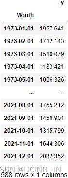

air = pd.read_csv(path+'air_passenger.csv',
                  index_col='date',
                  parse_dates=True
                 )
air.columns = ['y'] # rename 'passengers' to 'y'
air

Then, add the proper frequency for each DataFrame:

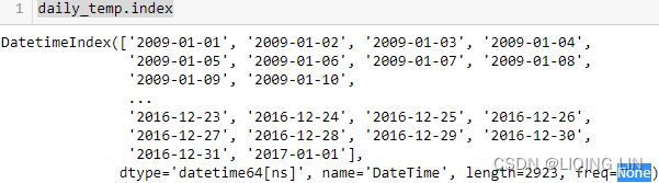
daily_temp.index.freq = 'D'
energy.index.freq = 'MS'
air.index.freq = 'M'
air.index

You can plot the three DataFrames to gain an understanding of how they differ:

daily_temp.plot( title='Avg Daily Weather Temperature in C',
                 figsize=(10,5)
               )
energy.plot( title='Monthly Energy Consumption',
             figsize=(10,5)
           )
air.plot( title='Monthly Passengers',
          figsize=(10,5)
        )
plt.show()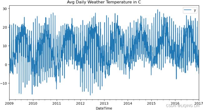

plotly_ts( ts_df=daily_temp, 
           title='Avg Daily Weather Temperature in C', 
           x_title='Date', y_title='Temperature in C' 
         )

Avg Daily Weather Temperature in C seem no trend, but exists repeating seasonality (every summer)

plotly_ts( ts_df=energy, 
           title='Total Energy Consumed by the Residential Sector', 
           x_title='Month', y_title='Total Energy Consumed' 
         )

The time series plot for the energy DataFrame shows a positive (upward) trend and a repeating seasonality (every winter). The energy_consumption data is recorded monthly from January 1973 to December 2021 (588 months). The seasonal magnitudes and variations over time seem to be unsteady, 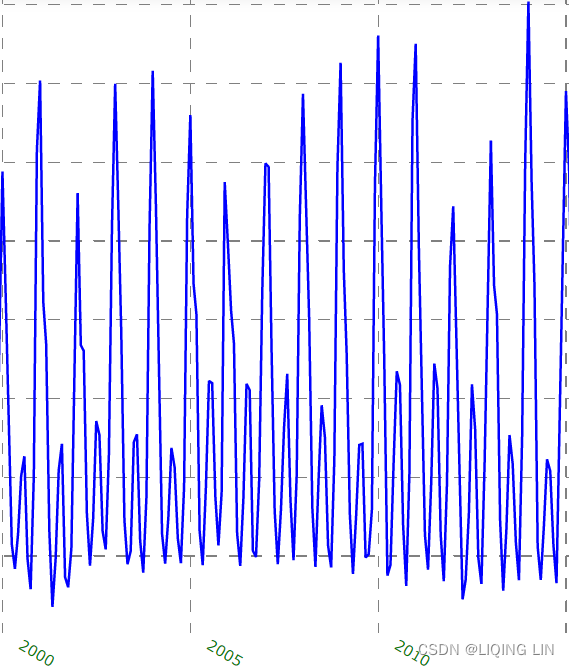indicating an multiple nature. Having a seasonal decomposition that specifes the level, trend, and season of an additive model will reflect this as well. For more insight on seasonal decomposition, please review the Decomposing time series data recipe in https://blog.csdn.net/Linli522362242/article/details/127737895, Exploratory Data Analysis and Diagnosis.

#############################

import plotly.graph_objects as go
 
def plotly_ts( ts_df, title, x_title='', y_title='' ):
    #hvplot.extension('plotly') # 'matplotlib' # 'bokeh' # holoviews
    # air.index[0] ==> Timestamp('1949-01-31 00:00:00', freq='M')
    start = pd.DatetimeIndex( ts_df.index ).year[0]
    end = pd.DatetimeIndex( ts_df.index ).year[-1]
 
    # https://stackoverflow.com/questions/59953431/how-to-change-plotly-figure-size
    layout=go.Layout(width=1000, height=500, 
                     title=f'{title} {start}-{end}',
                     title_x=0.5, title_y=0.9,
                     xaxis=dict(title=x_title, color='green', tickangle=30),
                     yaxis=dict(title=y_title, color='blue')
                    )
    fig = go.Figure(layout=layout)
    
    precision = 3
    fig.add_trace( go.Scatter( name='y', 
                               mode ='lines', 
                               line=dict(shape = 'linear', color = 'blue', #'rgb(100, 10, 100)', 
                                         width = 2, #dash = 'dashdot'
                                        ),
                               x=ts_df.index, y=ts_df.y,
                               #hovertemplate = '%{xaxis_title}: %{x|%Y-%m-%d}
%{yaxis_title}: %{y:%.1f}',
                               hovertemplate='
'.join([ x_title + ': %{x|%Y-%m-%d}',
                                                           y_title + f": %{{y:.{precision}f}}",
                                                          '',
                                                         ]),
                               showlegend=True,
                             )
                 )
 
    fig.update_xaxes(showgrid=True, ticklabelmode="period", gridcolor='grey', griddash='dash')
    fig.update_yaxes(showgrid=True, ticklabelmode="instant", gridcolor='grey', griddash='dash')
 
    fig.update_layout( hoverlabel=dict( font_color='white',
                                        #bgcolor="black"
                                      ),
                       legend=dict( x=0,y=1, 
                                    bgcolor='rgba(0,0,0,0)',#None
                                  ),
                       plot_bgcolor='rgba(0,0,0,0)',
                       #paper_bgcolor='rgba(0,0,0,0)',
                     )
 
    fig.show()
    
plotly_ts( ts_df=air, 
           title='Monthly Airline Passenger Numbers', 
           x_title='Date', y_title='#Passenger' 
         )

Figure 9.13 – The Air Passengers dataset showing trend and increasing seasonal variation

The air passenger data shows a long-term linear (upward) trend and seasonality. However, the seasonality fluctuations seem to be increasing as well, indicating a multiplicative model(A multiplicative model is suitable when the seasonal variation fluctuates over time. OR When the variation in the seasonal pattern, or the variation around the trend-cycle, appears to be proportional to the level of the time series与时间序列的水平成正比时, then a multiplicative decomposition is more appropriate. ).==>

#############################

When plotting the datasets, observe how each time series exhibits different characteristics(Trend,Seasonality, stationary). This initial insight will be helpful as you as proceed with the recipes in the chapter. In addition, you will realize how an algorithm's performance will vary when applied to different time series data.

Understanding supervised machine learning

In supervised machine learning, the data used for training contains known past outcomes, referred to as dependent or target variable(s). These are the variables you want your machine learning (ML) model to predict. The ML algorithm learns from the data using all other variables, known as independent or predictor variables, to determine how they are used to estimate the target variable. For example, the target variable is the house price in the house pricing prediction problem. The other variables, such as the number of bedrooms, number of bathrooms, total square footage/ˈfʊtɪdʒ/尺码长度, and city, are the independent variables used to train the model. You can think of the ML model as a mathematical model for making predictions on unobserved outcomes.

On the other hand, in unsupervised machine learning, the data contains no labels or outcomes to train on (unknown or unobserved). Unsupervised algorithms are used to find patterns in the data, such as the case with clustering, for example, customer segmentation, anomaly detection, or recommender systems.

Generally, there are two types of supervised machine learning: classification and regression.

In classifcation, the goal is to predict which class (or label) a particular observation belongs to. In other words, you are predicting a discrete value,
- for example, whether an email is spam or not spam or whether a transaction is fraudulent or not. The two examples represent a binary classification problem, but you can have a multi-class classification problem, such as the case with image classification.
- Some popular classification algorithms include Logistic Regression, Random Forests, K-Nearest Neighbors, and Support Vector Machines, to name a few.
In regression, you predict a continuous variable, such as the price of a house or a person's height. In regression,
- you can have a simple linear regression problem with one independent variable and one target variable,
- a multiple regression problem with more than one independent variable and one target variable,
- or a multivariate multiple regression problem with more than one independent variable and more than one dependent variable.
- Some popular linear regression algorithms include Linear Regression, Lasso Regression, and Elastic Net Regression. These examples are considered linear algorithms that assume a linear relationship between the variables.

Interestingly, several of the classification algorithms mentioned earlier can be used for regression; for example, you can have a Random Forest Regression, K-Nearest Neighbors Regression, and Support Vector Machines Regression. These regressors can capture non-linear relationships and produce more complex models.

Preparing time series data for supervised learning

In supervised ML, you must specify the independent variables (predictor variables) and the dependent variable (target variable). For example, in scikit-learn, you will use the fit(X, y) method for fitting a model, where X refers to the independent variable and y to the target variable.

Generally, preparing the time series data is similar to what you have done in previous chapters. However, additional steps will be specific to supervised ML, which is what this recipe is about. The following highlights the overall steps:

1. Inspect your time series data to ensure there are no significant gaps没有明显的差距, such as missing data, in your time series. If there are gaps, evaluate the impact and consider some of the imputation and interpolation techniques discussed in https://blog.csdn.net/Linli522362242/article/details/128422412, Handling Missing Data.
2. Understand any stationarity assumptions in the algorithm before fitting the model. If stationarity is an assumption before training, then transform the time series using the techniques discussed in the Detecting time series stationarity section in https://blog.csdn.net/Linli522362242/article/details/127737895, Exploratory Data Analysis and Diagnosis.
3. Transform your time series to contain independent and dependent variables. To do this, you will define a sliding window to convert the data into a window of inputs. For example, if you decide that the past five periods (lags) should be used to predict the current period (the sixth), then you will create a sliding window of five periods. This will transform a univariate time series into a tabular format. A univariate time series has only one dependent variable and no independent variables. For example, a five-period sliding window will produce five independent variables , , , , , which are lagged versions of the dependent variable. This representation of multiple inputs (a sequence) to one output is referred to as a one-step forecast. This will be the focus of this recipe. Figure 12.1 illustrates this concept.
4. Before training a model, split that data into training and test sets. Sometimes, you may need to split it into training, validation, and test sets, as you will explore in Chapter 13, Deep Learning for Time Series Forecasting.
5. Depending on the algorithm, you may need to scale your data; for example, in scikit-learn, you can leverage the StandardScaler(cp4 Training Sets Preprocessing_StringIO_dropna_categorical_feature_Encode_Scale_L1_L2_bbox_to_ancho_LIQING LIN的博客-CSDN博客center the feature columns at mean $\large \mu_x$ with standard deviation $\large \sigma_x$ so that the feature columns takes the form of a normal distribution) or the MinMaxScaler(this normalization refers to the rescaling of the features to a range of [0, 1]) class When making your predictions, you will need to inverse the transform to restore the results to their original scale, for example, you can use the inverse_transform method from scikit-learn.

In this recipe, you will prepare time series data for supervised learning by creating independent variables from a univariate time series. The following illustrates how a sliding window of five periods creates the dependent (target) variable at a time (t) and five independent variables ( , , , , , which are lagged versions of the dependent variable). In the daily temperature data, this means a five-day sliding window. Figure 12.1 – Example of a five-day sliding window for daily temperature data

Since you will be transforming all three DataFrames, you will create functions to simplify the process:

1. Inspect for missing data in the DataFrames. If there is missing data, then perform a simple fill forward imputation. First, make a copy so you do not change the original

air_copy = air.copy(deep=True)
energy_copy = energy.copy(deep=True)
daily_temp_copy = daily_temp.copy(deep=True)

Create the handle_missing_data function:

def handle_missing_data(df, ifreport=False):
    n = int( df.isna().sum() )
    if n>0:
        df.ffill(inplace=True)
        print( f'found\033[1m {n} missing\033[0m observations...', 
               end="" if ifreport else '\n'
             )
        if ifreport:
            return True

Pass each DataFrame to the handle_missing_data function:

for name, df in {'air_copy':air_copy, 
                 'energy_copy':energy_copy, 
                 'daily_temp_copy':daily_temp_copy
                }.items():
    
    if handle_missing_data(df, True):
        print(f'in \033[1m{name}\033[0m')

Only the daily_weather DataFrame had two NaN (missing values).

daily_temp_copy.isna().sum()

2. Create the create_lagXs_y function, which returns a DataFrame with a specified number of independent variables (columns) and a target variable (column). The total number of columns returned is based on the sliding window parameter (number of columns = sliding window + 1). This is illustrated in Figure 12.2. This technique was described in Machine Learning Strategies for Time Series Forecasting, Lecture Notes in Business Information Processing. Berlin, Heidelberg: Springer Berlin Heidelberg (https: //doi.org/10.1007/978-3-642-36318-4_3) . Create the function using the following:

The create_lagXs_y function, you produced additional columns to represent independent variables used in model training. The new columns are referred to as features. The process of engineering these new features, as you did earlier, is called feature engineering. In this, you create new features (columns) that were not part of the original data to improve your model's performance.

def create_lagXs_y( df, lag_window ):
    n = len(df)
    ts = df.values
    Xs = []
    idx = df.index[:-lag_window]
    # slice and draw
    for start in range( n-lag_window ):
        end = start + lag_window
        Xs.append( ts[start:end] ) # [x_0, x_1, x_2, x_3, x_4]
    cols = [ f'x_{i}' 
             for i in range(1, 1+lag_window)
           ]# columnName:[x_1, x_2, x_3, x_4, x_5]
    Xs = np.array(Xs).reshape(n-lag_window, -1) #==>shape:(n-lag_window, 5)
    y = df.iloc[lag_window:].values
    df_Xs = pd.DataFrame( Xs, columns=cols, index=idx )
    df_y = pd.DataFrame( y.reshape(-1), columns=['y'], index=idx )
    return pd.concat([df_Xs, df_y], 
                     axis=1
                    ).dropna()

The create_lagXs_y function will transform a time series with a specifed number of steps (the sliding window size).

For simplicity, transform all three DataFrames with the same sliding window size of five periods, lag_window=5 . Recall, the weather data is daily, so one period represents one day, while for the air passenger and energy consumption datasets, a period is equivalent to one month:

air_5_1 = create_lagXs_y( air_copy, 5 )
energy_5_1 = create_lagXs_y( energy_copy, 5 )
daily_temp_5_1 = create_lagXs_y( daily_temp_copy, 5 )

print( air_5_1.shape )
print( energy_5_1.shape )
print( daily_temp_5_1.shape )

air_5_1

3. You will need to split the data into training and test sets. You could use the train_test_split function from scikit-learn with shuffle=False . An alternative is to create the split_data function to split the data:

def split_data( df, test_split=0.15 ):
    n = int( len(df) * test_split )
    train, test = df[:-n], df[-n:]
    return train, test

The following shows how to use the split_data function:

train, test = split_data( air_5_1 )
print( f'Train: {len(train)} Test: {len(test)}' )

4. Certain algorithms benefit from scaling the data. You can use the StandardScaler class from scikit-learn. In this recipe, you will create the Standardize class with three methods: the fit_transform method, will fit on the training set and then transforms both the training and test sets, the inverse method is used to return a DataFrame to its original scale and the inverse_y method to inverse the target variable (or a specific column and not the entire DataFrame):

class Standardize:
    def __init__( self, split=0.15 ):
        self.split = split
        
    def _transform( self, df ):
        return (df - self.mu)/self.sigma ### 
    
    def split_data( self, df ):
        n = int( len(df) * test_split )
        train, test = df[:-n], df[-n:]
        return train, test
    
    def fit_transform( self, train, test ):
        self.mu = train.mean()   ###
        self.sigma = train.std() ###
        
        train_s = self._transform(train)
        test_s = self._transform(test)
        return train_s, test_s
    
    def transform( self, df ):
        return self._transform( df )
    
    def inverse( self, df ):
        return (df*self.sigma)+self.mu
    
    def inverse_y( self, df ):
        return ( df*self.sigma[-1] )+self.mu[-1]

The following shows how you can use the Standardize class:

scaler = Standardize()
train_s, test_s = scaler.fit_transform( train, test )
train_s

train_original = scaler.inverse(train_s)
train_original

y_train_original = scaler.inverse_y( train_s['y'] )
y_train_original

The Standardize class also has additional methods, such as split_data for convenience.

You will be leveraging these functions in the recipes of this chapter for data preparation.

Preparing time series data for supervised learning is summarized in Figure 12.1 and Figure 12.2. For example, in a regression problem, you are essentially transforming a univariate time series into a multiple regression problem. You will explore this concept further in the following One-step forecasting using linear regression models with scikit-learn recipe.

The lag_window parameter can be adjusted to fit your need. In the recipe, we used a split window of five (5) periods, and you should experiment with different window sizes.

The sliding window(lag_window) is one technique to create new features based on past observations. Other techniques can be used to extract features from time series data to prepare it for supervised machine learning. For example, you could create new columns based on the date column, such as day of the week, year, month, quarter, season, and other date-time features.

The following is an example of engineering date time related features using pandas:

df = daily_temp.copy(deep=False)
df

df = daily_temp.copy(deep=False)

df['day_of_week'] = df.index.dayofweek
df['days_in_month'] = df.index.days_in_month
df['month_end'] = df.index.is_month_end.astype(int)
df['is_leap'] = df.index.is_leap_year.astype(int)
df['month'] = df.index.month

df

Even though you will be using the create_lagXs_y function throughout the chapter, you should explore other feature engineering techniques and experiment with the different algorithms introduced in this chapter.

One-step forecasting using linear regression models with scikit-learn

In ts10_Univariate TS模型_circle mark pAcf_ETS_unpack product_darts_bokeh band interval_ljungbox_AIC_BIC_LIQING LIN的博客-CSDN博客ts10_2Univariate TS模型_pAcf_bokeh_AIC_BIC_combine seasonal_decompose twinx ylabel_bold partial title_LIQING LIN的博客-CSDN博客_first-order diff, Building Univariate Time Series Models Using Statistical Methods, you were introduced to statistical models such as AutoRegressive (AR $y_t= \beta_0 + \sum_{p=1}^{P}\beta_p y_{t-p} + \epsilon_t$ or $\large y_t= \beta_0 + \beta_1y_{t-1} + \beta_2y_{t-2} + \epsilon_t$ ) type models. These statistical models are considered linear models, where the independent variable(s) are lagged versions of the target (dependent) variable. In other words, the variable you want to predict is based on past values of itself at some lag.

In this recipe, you will move from statistical models into ML models. More specifically, you will be training different linear models, such as

Linear Regression
https://blog.csdn.net/Linli522362242/article/details/111307026
Simple linear regression :
The goal of simple (univariate) linear regression is to model the relationship between a single feature (explanatory variable, x) and a continuous-valued target (response variable, y).
Multiple linear regression :
OR
Here, is the y axis intercept with = 1.
$\large y$ or $\large y_t$ is the predicted variable,
or $\beta_0$ or is the intercept,
are the features or independent variables, and
$(\theta_1,\theta_2, ..., \theta_n)$ or $(\beta_1, \beta_2, ..., \beta_p)$ are the coefficients for each of the independent variables.
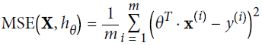
Mean Squared Error cost function:note $w_i == \theta_i$
Huber Regression https://blog.csdn.net/Linli522362242/article/details/107294292
Huber loss :
Suppose you want to train a regression model, but your training set is a bit noisy. Of course, you start by trying to clean up your dataset by removing or fixing the outliers, but that turns out to be insufficient; the dataset is still noisy. Which loss function should you use?
The Mean Squared Error might penalize large errors too much and cause your model to be imprecise.
The Mean Absolute Error $\left |y-f(x) \right |$ would not penalize outliers as much不会对异常值造成太大的惩罚, but training might take a while to converge, and the trained model might not be very precise. This is probably a good time to use the Huber loss

The Huber loss is quadratic when the error is smaller than a threshold δ (typically 1) but linear when the error is larger than δ. The linear part makes it less sensitive to outliers than the Mean Squared Error, and the quadratic part allows it to converge faster and be more precise than the Mean Absolute Error $\left |y-f(x) \right |$ ) instead of the good old MSE. The Huber loss is not currently part of the official Keras API, but it is available in tf.keras (just use an instance of the keras.losses.Huber class).
The three regression models, ElasticNet, Lasso, and Ridge, add a regularization (penalization) term to the objective function(cost function or loss function) that we want to minimize.
Regularization helps avoid overfitting during training and allows the model to better
generalize. Additionally, L1 regularization can be used for feature selection.
we can think of regularization as adding a penalty term to the cost function to encourage smaller weights; or, in other words, we penalize large weights.
Thus, by increasing the regularization strength via the regularization parameter $\large \lambda$ , we shrink the weights towards zero and decrease the dependence of our model on the training data.
Ridge Regression
Equation 4-8. Ridge Regression cost function
vs
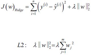
use RSS(Residuals of Sum Squares) instead of MSE
$\frac{1}{2}$ is for convenient computation, we should remove it for Practical application
L2 norm: $\sqrt{\sum_{i=1}^{n} \theta_i^2}$ OR $\sqrt{\sum_{j=1}^{m} w_j^2}$ e.g.
In Ridge Regression, the regularization term is referred to as L2 regularization and can shrink the coefficients of the least important features but does not eliminate them (no zero coefficients).
Under the penalty constraint, our best effort is to choose the point where the L2 ball intersects with the contours of the unpenalized cost function. The larger the value of the regularization parameter $\large \lambda$ gets, the faster the penalized cost function grows, which leads to a narrower L2 ball. For example, if we increase the regularization parameter $\large \lambda$ towards infinity, the weight coefficients will become effectively zero, denoted by the center of the L2 ball. To summarize the main message of the example: our goal is to minimize the sum of the unpenalized cost function plus the penalty term, which can be understood as adding bias and preferring a simpler model to reduce the variance(try to underfit) in the absence of sufficient training data to fit the model.
https://blog.csdn.net/Linli522362242/article/details/108230328
cp4 Training Sets Preprocessing_StringIO_dropna_categorical_feature_Encode_Scale_L1_L2_bbox_to_ancho_LIQING LIN的博客-CSDN博客
Equation 4-9. Ridge Regression closed-form solution
Note: Normal Equation(a closed-form equation)
Here is how to perform Ridge Regression with Scikit-Learn using a closed-form solution (a variant of Equation 4-9 using a matrix factorization technique by André-Louis Cholesky):

04_TrainingModels_Normal Equation(正态方程,正规方程) Derivation_Gradient Descent_Polynomial Regression_LIQING LIN的博客-CSDN博客
Lasso Regression
Equation 4-10. Lasso Regression cost function
vs
use RSS(Residuals of Sum Squares) instead of MSE
L1 norm: $\sqrt{\sum_{i=1}^{n} \left |\theta_i \right |}$ OR $\sqrt{\sum_{j=1}^{m} \left |w_j \right |}$ e.g.
In Lasso Regression, the regularization term can reduce the coefficient (the $\large w_j$ or $\large \theta_i$ in the objective function) of the least important features (independent variables) to zero, and thus eliminating them.
This added penalization term is called L1 regularization.
In the preceding figure, we can see that the contour of the cost function touches the L1 diamond at . Since the contours of an L1 regularized system are sharp, it is more likely that the optimum—that is, the intersection between the ellipses of the cost function and the boundary of the L1 diamond—is located on the axes, which encourages sparsity. The mathematical details of why L1 regularization can lead to sparse solutions are beyond the scope of this book. If you are interested, an excellent section on L2 versus L1 regularization can be found in section 3.4 of The Elements of Statistical Learning, Trevor Hastie, Robert Tibshirani, and Jerome Friedman, Springer.

The Lasso cost function is not differentiable无法进行微分运算 at $\theta_i = 0$ (for i = 1, 2, ⋯, n), but Gradient Descent still works fine if you use a subgradient vector g instead when any $\theta_i = 0$ . Equation 4-11 shows a subgradient vector equation you can use for Gradient Descent with the Lasso cost function.
Equation 4-11. Lasso Regression subgradient vector

04_TrainingModels_02_regularization_L2_cost_Ridge_Lasso_Elastic Net_Early Stopping_LIQING LIN的博客-CSDN博客
Elastic Net Regression
Elastic Net is a middle ground between Ridge Regression and Lasso Regression. The regularization term is a simple mix of both Ridge and Lasso’s regularization terms, and you can control the mix ratio r. When r = 0, Elastic Net is equivalent to Ridge Regression, and when r = 1, it is equivalent to Lasso Regression (see Equation 4-12).

Equation 4-12. Elastic Net cost function
ElasticNet Regression, on the other hand, is a hybrid between the two by combining L1 and L2 regularization terms.
other loss function:mpf11_Learning rate_Activation_Loss_Optimizer_Quadratic Program_NewtonTaylor_L-BFGS_Nesterov_Hessian_LIQING LIN的博客-CSDN博客_standardscaler activation function

These are considered linear regression models and assume a linear relationship between the variables.

In the previous recipe, you transformed a univariate time series into a multiple regression problem with five independent variables and one dependent variable (a total of six columns), as shown in the following diagram:Figure 12.2 – Transforming time series for supervised ML

For the representation in Figure 12.2, the multiple linear regression equation would be as follows:
$\large \hat{y} = \beta_0 + \beta_1x_1 + \beta_2x_2 +... +\beta_5 x_5 + \epsilon$

Where $\hat{y}$ is the estimated (predicted) value, ( $\beta_1$ , $\beta_2$ ,..., $\beta_5$ ) are the coefficients for each
independent variable (, , , , ), $\beta_0$ is the intercept, and ϵ is the residual or error
term. Remember, the independent variables that were created (, , , , ) are lagged
versions of the dependent variable ( ) created using a sliding window. You can simplify
the equation in matrix notation by adding an term, which is a constant value of one (
). This will give us the following equation:

$\large \hat{y} = \beta X + \epsilon$

In linear regression, you want to minimize the errors (loss), which is the difference between the actual value, $\large Y_i$ , and the estimated value, $\large \hat{y}_i$ . More specifically, it is the square loss at each data point. If we take the sum of these squared losses or errors, you get the Residual Sum of Square (RSS). The cost function (RSS) is what you want to minimize. This results in our objective function being written as follows:
$\large min \sum_{i=1}^{n} (Y_i - \sum_{j=0}^{m} \beta_j X_{i,j})^2$

Sometimes, you will see the objective function as minimizing the Mean Squared Error (MSE), which is obtained by dividing the RSS by the degrees of freedom (for simplicity, you can think of it as the number of observations, where N represents the number of elements. By default ddof is zerocp4 Training Sets Preprocessing_StringIO_dropna_categorical_feature_Encode_Scale_L1_L2_bbox_to_ancho_LIQING LIN的博客-CSDN博客).

Once a time series is prepared for supervised ML, you can use any regression algorithm to train a model. This is summarized in Figure 12.2. The function for transforming the time series is create_lagXs_y( df, lag_window ), to remind you that we are preparing the data so that a sequence of inputs is given (the independent variables) to produce a single output (one-step forecast).

In this recipe, you will continue using the three DataFrames you loaded from the Technical requirements section of this chapter. You will leverage the functions and classes created in the previous Preparing time series data for supervised learning recipe.

Start by loading the necessary classes and functions for this recipe. Make a copy of the DataFrames to ensure they do not get overwritten:

from sklearn.linear_model import ( LinearRegression,
                                   ElasticNet,
                                   Ridge,
                                   Lasso,
                                   HuberRegressor
                                 )
air_cp = air.copy(deep=True)
en_cp = energy.copy(deep=True)
dw_cp = daily_temp.copy(deep=True)

The following steps will use the energy consumption data for demonstration. You should use the same steps on all three DataFrames, as shown in the accompanying Jupyter notebook:

1. Use the handle_missing_data function to ensure there are no missing values:

for name, df in {'air_copy':air_cp, 
                 'energy_copy':en_cp, 
                 'daily_temp_copy':dw_cp
                }.items():
    
    if handle_missing_data(df, True):
        print(f'in \033[1m{name}\033[0m')

dw_cp.isna().sum()

2. Use create_lagXs_y to convert the time series DataFrames into a supervised learning problem with 10 steps (windows):

air_10_1 = create_lagXs_y( air_cp, 10 )
energy_10_1 = create_lagXs_y( en_cp, 10 )
daily_temp_10_1 = create_lagXs_y( dw_cp, 10 )

print( air_10_1.shape )
print( energy_10_1.shape )
print( daily_temp_10_1.shape )

Feel free to change the window size.

3. Split and scale the data using the split_data function and the Standardize class. Later, you can use the class instance to inverse the scaling:

train_air, test_air = split_data( air_10_1, test_split=0.10 )

scaler_air = Standardize()
train_air_s, test_air_s = scaler_air.fit_transform( train_air, test_air )

train_air_s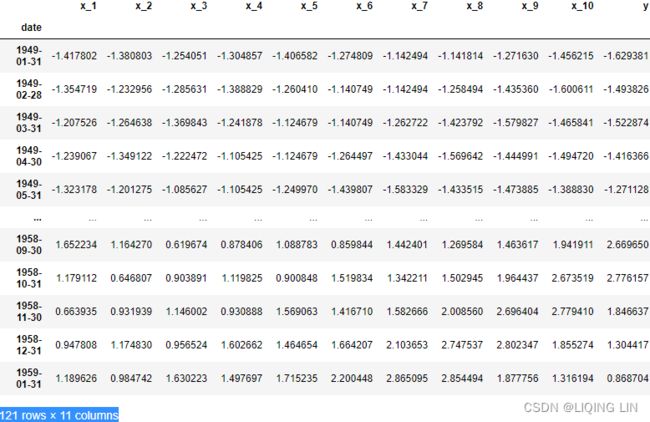

train_en, test_en = split_data( energy_10_1, test_split=0.10 )

scaler_en = Standardize()
train_en_s, test_en_s = scaler_en.fit_transform( train_en, test_en )

train_en_s

train_dw, test_dw = split_data( daily_temp_10_1, test_split=0.10 )

scaler_dw = Standardize()
train_dw_s, test_dw_s = scaler_dw.fit_transform( train_dw, test_dw )

train_dw_s

Common error metrics used in regression are Mean Squared Error(MSE) or Root Mean Squared Error(RMSE). These are scale-dependent, so if you experiment with different model configurations, for example, scale your data using the Standardize class function, this will impact the scores and make it difficult to compare.

MAPE(Mean Absolute Percentage Error)

Another popular error metric in forecasting is Mean Absolute Percentage Error(MAPE), which is more intuitive to interpret since it is expressed as a percentage and is scale-independent与数据的比例无关. For certain problems, MAPE may not be suitable. For example, with the daily temperature data, MAPE puts a heavier penalty on negative errors (you can have negative Celsius). With MAPE, you cannot divide by zero (Celsius at zero can be problematic). Additionally, measuring temperature as a percentage may not make sense in this case.

The Mean Absolute Percentage Error(MAPE), also known as Mean Absolute Percentage Deviation (MAPD), is a measure of prediction accuracy of a forecasting method in statistics. It usually expresses the accuracy as a ratio defined by the formula: $\large MAPE = \frac{100%}{n} \sum_{t=1}^{n} \left | \frac{A_t - F_t}{A_t} \right |$ where $\large A_t$ is the actual value and $\large F_t$ is the forecast value. Their difference is divided by the actual value $\large A_t$ . The absolute value of this ratio is summed for every forecasted point in time and divided by the number of fitted points n.

It's a good practice to capture different metrics, and in this case, you will capture both RMSE and MAPE by importing them from sktime . Note that sklearn does support both MSE and MAPE. The third metric, which has been proposed as an alternative to the shortcoming of MAPE, is the Mean Absolute Scaled Error (MASE) metric.

def _percentage_error(y_true, y_pred, symmetric=True):
    """Percentage error.
    Parameters
    ----------
    y_true : pd.Series, pd.DataFrame or np.array of shape (fh,) or (fh, n_outputs) \
             where fh is the forecasting horizon
        Ground truth (correct) target values.
    y_pred : pd.Series, pd.DataFrame or np.array of shape (fh,) or (fh, n_outputs) \
             where fh is the forecasting horizon
        Forecasted values.
    symmetric : bool, default = False
        Whether to calculate symmetric percentage error.
    Returns
    -------
    percentage_error : float
    References
    ----------
    Hyndman, R. J and Koehler, A. B. (2006). "Another look at measures of \
    forecast accuracy", International Journal of Forecasting, Volume 22, Issue 4.
    """
    if symmetric:
        # Alternatively could use np.abs(y_true + y_pred) in denom
        # Results will be different if y_true and y_pred have different signs
        percentage_error = (
            2
            * np.abs(y_true - y_pred)
            / np.maximum( np.abs(y_true) + np.abs(y_pred), EPS )
        ) # note : EPS = np.finfo(np.float64).eps
    else:
        percentage_error = (y_true - y_pred) / np.maximum(np.abs(y_true), EPS)
    return percentage_error


def mean_absolute_percentage_error(
    y_true,
    y_pred,
    horizon_weight=None,
    multioutput="uniform_average",
    symmetric=True,
    **kwargs,
):
#https://github.com/sktime/sktime/blob/4e06cb0231cdabb74bf88d0cb4f2b721fc863fe3/sktime/performance_metrics/forecasting/_functions.py#L1447 

    output_errors = np.average(
        np.abs(_percentage_error(y_true, y_pred, symmetric=symmetric)),
        weights=horizon_weight, # default None
        axis=0,
    )

SMAPE(Symmetric Mean Absolute Percentage Error)

Symmetric Mean Absolute Percentage Error (SMAPE or sMAPE) is an accuracy measure based on percentage (or relative) errors. It is usually defined[citation needed] as follows: $\large {\color{Blue} s}MAPE_{1st} = \frac{100%}{n} \sum_{t=1}^{n} \frac{\left |A_t - F_t \right |}{(\left |A_t \right |+ \left |F_t \right | )/2} = \frac{100%}{n} \sum_{t=1}^{n} \frac{\left |F_t - A_t \right |}{(\left |A_t \right |+ \left |F_t \right | )/2}$ sktime
The absolute difference between $\large A_t$ and $\large F_t$ is divided by half the sum of absolute values of the actual value $\large A_t$ and the forecast value $\large F_t$ . The value of this calculation is summed for every fitted point $\large t$ and divided again by the number of fitted points $\large n$ .

The earliest reference to similar formula appears to be Armstrong (1985, p. 348) where it is called "adjusted MAPE" and is defined without the absolute values in denominator. It has been later discussed, modified and re-proposed by Flores (1986).

Armstrong's original definition is as follows: $\large {\color{Blue} s}MAPE = \frac{1}{n} \sum_{t=1}^{n} \frac{\left |F_t - A_t \right |}{(A_t + F_t )/2}$

The problem is that it can be negative (if $A_{t}+F_{t}<0$ ) or even undefined (if $A_{t}+F_{t}=0$ ). Therefore the currently accepted version of SMAPE assumes the absolute values in the denominator(sktime solved them by using EPS).

In contrast to the (MAPE) mean absolute percentage error, SMAPE has both a lower bound and an upper bound. Indeed, the formula above provides a result between 0% and 200%. However a percentage error between 0% and 100% is much easier to interpret. That is the reason why the formula below is often used in practice (i.e. no factor 0.5 OR $\small /2$ in denominator): $\large {\color{Blue} s}MAPE_{2nd} = \frac{100%}{n} \sum_{t=1}^{n} \frac{\left |A_t - F_t \right |}{\left |A_t \right |+ \left |F_t \right | } = \frac{100%}{n} \sum_{t=1}^{n} \frac{\left |F_t - A_t \right |}{\left |A_t \right |+ \left |F_t \right | }$

In the above formula, if $\large A_{t}=F_{t}=0$ , then the t'th term in the summation is 0, since the percent error between the two is clearly 0 两者之间的百分比误差显然为 0 and the value of $\large {\frac {|0-0|}{|0|+|0|}}$ is undefined.

One supposed problem with SMAPE is that it is not symmetric since over- and under-forecasts are not treated equally. This is illustrated by the following example by applying the second SMAPE formula $\large {\color{Blue} s}MAPE_{2nd} = \frac{100%}{n} \sum_{t=1}^{n} \frac{\left |A_t - F_t \right |}{\left |A_t \right |+ \left |F_t \right | } = \frac{100%}{n} \sum_{t=1}^{n} \frac{\left |F_t - A_t \right |}{\left |A_t \right |+ \left |F_t \right | }$ :

Over-forecasting: At = 100 and Ft = 110 give SMAPE = 4.76%
Under-forecasting: At = 100 and Ft = 90 give SMAPE = 5.26%.

However, one should only expect this type of symmetry for measures which are entirely difference-based and not relative (such as mean squared error and mean absolute deviation). 但是，对于完全基于差异而非相对的度量（例如均方误差和平均绝对偏差），应该只期望这种类型的对称性。

There is a third version of SMAPE, which allows to measure the direction of the bias in the data by generating a positive and a negative error on line item level. Furthermore it is better protected against outliers and the bias effect更好地防止异常值和偏差效应 mentioned in the previous paragraph than the two other formulas. The formula is: $\large sMAPE_{3rd Version} = \frac{\sum_{t=1}^{n} \left |F_t-A_t \right | }{\sum_{t=1}^{n}(A_t+F_t)}$
A limitation to SMAPE is that if the actual value or forecast value is 0, the value of error will boom up to the upper-limit of error. (200% for the first formula and 100% for the second formula).

Provided the data are strictly positive, a better measure of relative accuracy can be obtained based on the log of the accuracy ratio: log(Ft / At) This measure is easier to analyse statistically, and has valuable symmetry and unbiasedness properties. When used in constructing forecasting models the resulting prediction corresponds to the geometric mean (Tofallis, 2015).

MASE

The mean absolute scaled error has the following desirable properties:[3]

Scale invariance: The Mean Absolute Scaled Error is independent of the scale of the data与数据的比例无关, so can be used to compare forecasts across data sets with different scales.
MASE is independent of the scale of the forecast since it is defined using ratio of errors in the forecast. This means MASE values will be similar if we are forecasting high valued time series like number of internet traffic packet crossing a router hourly when compared to forecasting number of pedestrians crossing a busy traffic light every hour.
Predictable behavior as $\large A_{t}\rightarrow 0$ or $\large o_{t}\rightarrow 0$ : Percentage forecast accuracy measures such as the Mean absolute percentage error (MAPE $\large MAPE = \frac{100%}{n} \sum_{t=1}^{n} \left | \frac{A_t - F_t}{A_t} \right | = \frac{100%}{T} \sum_{t=1}^{T} \left | \frac{o_t - F_t}{o_t} \right |$ ) rely on division of $\large A_t$ , skewing the distribution of the MAPE for values of $\large A_t$ near or equal to 0. This is especially problematic for data sets whose scales do not have a meaningful 0, such as temperature in Celsius or Fahrenheit, and for intermittent/ˌɪntərˈmɪtənt/间歇的,断断续续的 demand data sets, where occurs frequently.
MASE is immune to the problem不受...问题的影响 faced by Mean Absolute Percentage Error (MAPE) when actual time series output $\large A_t$ or $\large o_t$ or at any time step is zero(since the denominator is the mean absolute error of the one-step "naive forecast method" on the training set). In this situation MAPE gives an infinite output, which is not meaningful. However, it is noted that for a time series with all values equal to zero at all steps, MASE output will also be not defined but such time series are not realistic.
Symmetry: The Mean Absolute Scaled Error
penalizes positive and negative forecast errors equally, and
penalizes errors in large forecasts and small forecasts equally. In contrast, the MAPE and median absolute percentage error (MdAPE) fail both of these criteria, while the "symmetric" sMAPE and sMdAPE[4] fail the second criterion.
Interpretability: The Mean Absolute Scaled Error can be easily interpreted, as values greater than one(>1) indicate that in-sample one-step forecasts from the naïve method perform better than the forecast values under consideration.

Mean Absolute Error (MAE) for the predictions from the algorithm $\large o_i$ : actual value, $\large y_i$ : predction
Its value greater than one (1) indicates the algorithm is performing poorly compared to the naïve forecast.
Asymptotic normality of the MASE: The Diebold-Mariano test for one-step forecasts is used to test the statistical significance of the difference between two sets of forecasts.[5][6][7] To perform hypothesis testing with the Diebold-Mariano test statistic, it is desirable for $DM\sim N(0,1)$ , where is the value of the test statistic. The DM statistic for the MASE has been empirically shown to approximate this distribution, while the Mean Relative Absolute Error (MRAE), MAPE and sMAPE do not.

Non seasonal time series

For a non-seasonal time series,[8] the Mean Absolute Scaled Error is estimated by $\large MASE = mean(\frac{\left |e_j \right |}{\frac{1}{T-1}\sum_{t=2}^{T}\left | Y_t - Y_{t-1} \right|}) = \frac{\frac{1}{J}\sum_{j}^{}\left | e_j \right |}{\frac{1}{T-1}\sum_{t=2}^{T}\left | Y_t - Y_{t-1} \right|}$
where the numerator $\large e_j$ is the forecast error for a given period (with $\large J$ , the number of forecasts), defined as the actual value ( $\large Y_j$ ) minus the forecast value ( $\large F_j$ ) for that period: $\large e_j = Y_j - F_j$ , and the denominator is the mean absolute error of the one-step "naive forecast method" on the training set (here defined as t = 1..T),[8] which uses the actual value from the prior period as the forecast: $\large F_t = Y_{t-1}$
#########

1. Calculate Mean Absolute Error (MAE) for the predictions from the algorithm

$\large o_i$ : actual value
Consider a time series with output(forecast or prediction) for N steps given as y1, y2, y3,…yn

(the denominator )Naïve forecast error at different time steps is given by:
(the denominator )Mean Absolute Error for naïve forecast over entire duration is defined as

2. MASE is given by the ratio of MAE for algorithm and MAE of naïve forecast.

#########

Seasonal time series

For a seasonal time series, the Mean Absolute Scaled Error is estimated in a manner similar to the method for non-seasonal time series: $\large MASE = mean(\frac{\left |e_j \right |}{\frac{1}{T-m}\sum_{t=m+1}^{T}\left | Y_t - Y_{t-m} \right|}) = \frac{\frac{1}{J}\sum_{j}^{}\left | e_j \right |}{\frac{1}{T-m}\sum_{t=m+1}^{T}\left | Y_t - Y_{t-m} \right|}$
The main difference with the method for non-seasonal time series, is that the denominator is the mean absolute error of the one-step "seasonal naive forecast method" on the training set,[8] which uses the actual value from the prior season as the forecast: $\large F_t = Y_{t-m}$ ,[9] where m is the seasonal period.

This scale-free error metric "can be used to compare forecast methods on a single series and also to compare forecast accuracy between series. This metric is well suited to intermittent-demand series[clarification needed] because it never gives infinite or undefined values[1] except in the irrelevant case where all historical data are equal.

When comparing forecasting methods, the method with the lowest MASE is the preferred method.

Seasonal variation in the forecast is captured by equating the current forecast to the actual output from the period in last season corresponding to current period, e.g. prediction of demand of a product in holiday season is made equal to the actual demand of the product from last holiday season.
(the denominator )Mean Absolute Error for naïve forecast over entire duration is defined as

Non-time series data

For non-time series data, the mean of the data ( $\large \bar {Y}$ ) can be used as the "base" forecast. $\large MASE = mean(\frac{\left |e_j \right |}{\frac{1}{J}\sum_{j=1}^{J}\left | Y_j - \bar{Y} \right|}) = \frac{\frac{1}{J}\sum_{j}^{}\left | e_j \right |}{\frac{1}{J}\sum_{j}^{}\left | Y_j - \bar{Y} \right|}$ In this case the MASE is the Mean absolute error divided by the Mean Absolute Deviation.

You will use MASE from the sktime library as well:

from sktime.performance_metrics.forecasting import( MeanSquaredError,
                                                    MeanAbsolutePercentageError,
                                                    MeanAbsoluteScaledError
                                                  )

Create an instance of each of the classes to use later in the recipe:

mse = MeanSquaredError()
mape = MeanAbsolutePercentageError()
mase = MeanAbsoluteScaledError()

Note, you will be calculating RMSE as the square root of MSE, for example, using
np.sqrt( mse(y_actual – y_hat) ) .

4. Create the train_model function that takes the training and test sets, then fits the model on the train set and evaluates the model using the test set using
MAPE( $\large MAPE = \frac{100%}{n} \sum_{t=1}^{n} \left | \frac{A_t - F_t}{A_t} \right |$ ),
MASE( $\large MASE = mean(\frac{\left |e_j \right |}{\frac{1}{T-m}\sum_{t=m+1}^{T}\left | Y_t - Y_{t-m} \right|}) = \frac{\frac{1}{J}\sum_{j}^{}\left | e_j \right |}{\frac{1}{T-m}\sum_{t=m+1}^{T}\left | Y_t - Y_{t-m} \right|}$ ), and RMSE(). The function will return a dictionary with additional model information:

def train_model( train, test, regressor, reg_name ):
    X_train, y_train = train.drop( columns=['y'] ), train['y']
    X_test, y_test = test.drop( columns=['y'] ), test['y']
    
    print( f'training {reg_name} ...' )
    regressor.fit( X_train, y_train )
    
    yhat = regressor.predict( X_test )
    
    rmse_test = np.sqrt( mse(y_test, yhat) )
    mape_test = mape( y_test, yhat )
    mase_test = mase( y_test, yhat, y_train=y_train )
    
    residuals = y_test.values - yhat
    
    model_metadata = {'Model Name': reg_name, 'Model': regressor,
                      'RMSE': rmse_test,
                      'MAPE': mape_test,
                      'MASE': mase_test,
                      'yhat': yhat, 
                      'resid': residuals, 
                      'actual': y_test.values
                     }
    return model_metadata

The function returns the model and evaluation metrics against the test data, the forecast, and the residuals.

5. Create a dictionary that contains the regression algorithms and their names (keys) to use in a loop. This makes it easier later to update the dictionary with additional regressors:

regressors = { 'Linear Regression': LinearRegression(fit_intercept=False),
               # alpha:Constant that multiplies the penalty terms. and l1_ratio=0.5 Ridge + Lasso
               'Elastic Net': ElasticNet(alpha=0.5, fit_intercept=False), # False, the data is assumed to be already centered
               'Ridge Regression': Ridge(alpha=0.5, fit_intercept=False),
               'Lasso Regression': Lasso(alpha=0.5, fit_intercept=False),
               'Huber Regression': HuberRegressor(fit_intercept=False)
             }

The three regressors, Ridge, Lasso, and ElasticNet, add a regularization (penalization) term to the objective function. All three take an alpha ( α ) parameter, which determines the penalization factor for the coefficients. This is a hyperparameter you can experiment with; for now, you will use the value ( 0.5 ).

6. The train_model function fits and evaluates one model at a time. Create another function, train_different_models , which can loop through the dictionary of regressors and calls the train_model function. The function will return the results from each regressor as a list:

def train_different_models( train, test, regressors):
    results = []
    for reg_name, regressor in regressors.items():
        results.append( train_model( train,
                                     test,
                                     regressor,
                                     reg_name
                                   )
                      )
    return results

Pass the dictionary of regressors along with the training and test sets to the train_different_models function and store the results:

air_results = train_different_models( train_air_s, test_air_s, regressors )
en_results = train_different_models( train_en_s, test_en_s, regressors )
dw_results = train_different_models( train_dw_s, test_dw_s, regressors )

import warnings
warnings.filterwarnings('ignore')

air_results = train_different_models( train_air_s, test_air_s, regressors )
en_results = train_different_models( train_en_s, test_en_s, regressors )
dw_results = train_different_models( train_dw_s, test_dw_s, regressors )

en_results

7. You can convert the results into a DataFrame to view the scores and model name:

cols = ['Model Name', 'RMSE', 'MAPE', 'MASE']
air_results = pd.DataFrame( air_results )
air_results[cols].sort_values('MASE')

The preceding code should produce the following results:

en_results = pd.DataFrame( en_results )
en_results[cols].sort_values('MASE')

Figure 12.3 – Results of all five regression models on the energy consumption data

dw_results = pd.DataFrame( dw_results )
dw_results[cols].sort_values('MASE')

You can update the sort_values method to use RMSE or MAPE and observe any changes in the ranking. Note that you did not reset the index since the order (row ID) is aligned with the order from the regressors dictionary.

cols = ['yhat', 'resid', 'actual', 'Model Name']
for row in en_results[cols].iterrows():
    print(row)

8. The en_results list contains the actual test results ( actual ), the forecast value ( yhat ), and the residuals ( resid ). You can use these to visualize the model's performance. Create a plot_results function to help diagnose the models:

from statsmodels.graphics.tsaplots import plot_acf

def plot_results( cols, results, data_name ):
    for row in results[cols].iterrows():
        yhat, resid, actual, name = row[1] # row[0] : index
        #plt.figure(figsize=(10,6))
        plt.rcParams["figure.figsize"] = [10, 3]   ##
        plt.title( r'{} - $\bf{}$'.format(data_name, name) )
        plt.plot( actual, 'k--', alpha=0.5 )
        plt.plot( yhat, 'k' )
        plt.legend( ['actual', 'forecast'] )
        plot_acf(resid, zero=False,
                 title=f'{data_name} - Autocorrelation'
                )
        plt.show()

Notice the use of the plot_acf function from statsmodels to evaluate the residuals. The following is an example of using the plot_results function on the energy consumption data:

cols = ['yhat', 'resid', 'actual', 'Model Name']
plot_results(cols, en_results, 'Energy Consumption')

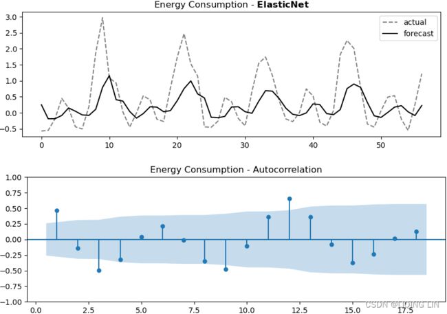
The preceding code should produce two plots for each of the five models (a total of 10 plots for the energy consumption data). For each model, the function will output a line plot comparing out-of-sample data (test data) against the forecast (predicted values) and a residual autocorrelation plot. Figure 12.4 – Hubber Regression plots

Observe from the plots how the models rank and behave differently on different time series processes.

From Figure 12.4, the Hubber Regression model seems to perform well with a potential for further tuning. Later in this chapter, you will explore hyperparameter tuning in the Optimizing a forecasting model with hyperparameter tuning recipe.

Later, in the Forecasting using non-linear models with sktime recipe, you will explore more regressors (linear and non-linear) and how to deal with trend and seasonality.

from statsmodels.graphics.tsaplots import plot_acf

def plot_resultMix( cols, results, data_name ):
    fig, ax = plt.subplots( figsize=(12,6) )
    
    color_list = ['orange', 'cyan', 'red', 'magenta', 'blue']
    alpha_list = [0.8,     1,        1,       0.5,        1]
    ls_list = [ 'o',     ':',     '--',     ':',        '--']
    
    for row in results[cols].iterrows():
        idx, (yhat, resid, actual, name) = row # row[0] : index
        # print(name, color_list[idx], idx)
        if idx==0:
            ax.plot( actual,
                     'k--', alpha=0.5,
                     label='actual',
                   )
            ax.plot( yhat, color=color_list[idx], alpha=alpha_list[idx], marker=ls_list[idx],
                     label=name
                   )
        else:    
            ax.plot( yhat, color=color_list[idx], alpha=alpha_list[idx], ls=ls_list[idx], 
                     label=name
                   )
        plt.rcParams["figure.figsize"] = [12, 2]   ##
        plot_acf(resid, zero=False,
                 #title=f'{name} Residual - Autocorrelation'
                 title = r' $\bf{}$ Residual - Autocorrelation'.format(name)
                )
    ax.set_title(r'$\bf{}$'.format(data_name))    
    ax.autoscale(enable=True, axis='x', tight=True)### ### Align both ends  
    ax.legend(fancybox=True, framealpha=0)
    plt.show()
        
cols = ['yhat', 'resid', 'actual', 'Model Name']
plot_resultMix(cols, en_results, 'Energy Consumption')

the Hubber Regression model seems to perform well with a potential for further tuning.

##############

plotly acf vlines

import plotly.graph_objects as go

def plotly_resultMix( cols, results, data_name, x_title='', y_title='' ):

    # https://stackoverflow.com/questions/59953431/how-to-change-plotly-figure-size
    layout=go.Layout(width=1000, height=600, 
                     title=f'{data_name}',
                     title_x=0.5, title_y=0.9,
                     #xaxis=dict(title=x_title, color='green', tickangle=30),
                     #yaxis=dict(title=y_title, color='blue')
                    )
    fig = go.Figure(layout=layout)
    
    color_list = ['orange', 'red', 'blue', 'magenta', 'black']
    #alpha_list = [0.8,           1,     1,       0.5,    1]
    lws = [         6,           2,     4,         2,    2]
    ls_list =[  'dot',       'dot','dash',     'dot', None]
    
    for row in results[cols].iterrows():
        idx, (yhat, resid, actual, name) = row # row[0] : index
        #print(name, color_list[idx], idx)
        
        if idx == 0 :
            fig.add_trace( go.Scatter( name='actual', 
                                       mode ='lines', 
                                       line=dict(shape = 'linear', color = 'firebrick', #'rgb(100, 10, 100)', 
                                                 width = 1, 
                                                 dash = 'dash'
                                                ),
                                       y=actual,
                                     )
                         )
        fig.add_trace( go.Scatter( name=name, 
                                   mode ='lines', 
                                   line=dict(shape = 'linear', color = color_list[idx], #'rgb(100, 10, 100)', 
                                             width = lws[idx], 
                                             dash = ls_list[idx],
                                            ),
                                   y=yhat,
                                 )
                    )

    fig.update_xaxes(showgrid=False, ticklabelmode="period", gridcolor='grey', griddash='dash')
    fig.update_yaxes(showgrid=False, ticklabelmode="instant", gridcolor='grey', griddash='dash')

    fig.update_layout( title_font_family="Times New Roman", title_font_size=30,
                       hoverlabel=dict( font_color='white',
                                        #bgcolor="black"
                                      ),
                       legend=dict( x=0.83,y=1, 
                                    bgcolor='rgba(0,0,0,0)',#None
                                  ),
                       plot_bgcolor='white',#"LightSteelBlue",#'rgba(0,0,0,0)',
                       #paper_bgcolor="LightSteelBlue",
                     )

    fig.show()
 
cols = ['yhat', 'resid', 'actual', 'Model Name']

plotly_resultMix( cols, 
                  results=en_results, 
                  data_name='Energy Consumption', 
                  # x_title='Date', y_title='#Passenger' 
                )

import plotly.graph_objects as go
from statsmodels.tsa.stattools import acf
from plotly.subplots import make_subplots
def plotly_resultMix( cols, results, data_name, x_title='', y_title='' ):

    # https://stackoverflow.com/questions/59953431/how-to-change-plotly-figure-size
    layout=go.Layout(width=1000, height=600, 
                     title=f'{data_name}',
                     title_x=0.5, title_y=0.9,
                     #xaxis=dict(title=x_title, color='green', tickangle=30),
                     #yaxis=dict(title=y_title, color='blue')
                    )
    fig = go.Figure(layout=layout)
    
    color_list = ['orange', 'red', 'blue', 'magenta', 'black']
    #alpha_list = [0.8,           1,     1,       0.5,    1]
    lws = [         6,           2,     4,         2,    2]
    ls_list =[  'dot',       'dot','dash',     'dot', None]
    
    ##########
    # https://plotly.com/python-api-reference/generated/plotly.subplots.make_subplots.html
    acf_plots = make_subplots(rows=len(en_results), cols=1,
                              shared_xaxes=True,
                              vertical_spacing=0.05,
                              subplot_titles=results['Model Name'],
                              #column_widths=[1000]*len(results),
                              row_heights=[1000]*len(results),
                             )
    ##########
    
    for row in results[cols].iterrows():
        idx, (yhat, resid, actual, name) = row # row[0] : index
        #print(name, color_list[idx], idx)
        
        if idx == 0 :
            fig.add_trace( go.Scatter( name='actual', 
                                       mode ='lines', 
                                       line=dict(shape = 'linear', color = 'firebrick', #'rgb(100, 10, 100)', 
                                                 width = 1, 
                                                 dash = 'dash'
                                                ),
                                       y=actual,
                                     )
                         )
        fig.add_trace( go.Scatter( name=name, 
                                   mode ='lines', 
                                   line=dict(shape = 'linear', color = color_list[idx], #'rgb(100, 10, 100)', 
                                             width = lws[idx], 
                                             dash = ls_list[idx],
                                            ),
                                   y=yhat,
                                 )
                     )

        ##########
        acf_x, confint_interval, _, _ =acf( resid, nlags=18, alpha=0.05,
                                            fft=False, qstat=True,
                                            #bartlett_confint=True,
                                            #adjusted=False,
                                            missing='none',
                                        )
                #lags=np.array(range(18))
        lags = np.arange(start=0, stop=acf_x.shape[0], dtype='float')

        #.scatter(x=xlabel, y=acf_value, c='red')
        acf_plots.add_trace( go.Scatter( name=name,
                                         mode='markers',
                                         x=lags[1:],
                                         y=acf_x[1:],
                                         line=dict(color=color_list[idx])
                                       ),
                             row=idx+1, col=1,
                           )
        acf_plots.add_hline( y=0,
                             line_width=1,
                             row=idx+1, col=1,
                           )
        # plot multiple  verical lines
        # print( np.repeat( np.array( lags[1:] ), 2 ).reshape(-1,2) )
        xx = np.repeat( np.array( lags[1:] ), 2 ).reshape(-1,2)
#         print( np.concatenate( ( np.zeros( len(acf_x[1:]) )[:, np.newaxis], np.array(acf_x[1:])[:, np.newaxis] ),
#                                axis=1
#                              )
#              )
        yy = np.concatenate( ( np.zeros( len(acf_x[1:]) )[:, np.newaxis], 
                               np.array(acf_x[1:])[:, np.newaxis] 
                             ),
                             axis=1
                           )
        for i in range(len(xx)):
            acf_plots.add_trace( go.Scatter( x=xx[i], y=yy[i], 
                                             mode='lines',
                                             line=dict(color=color_list[idx])
                                           ),
                                 row=idx+1, col=1,
                               )
        
        lags[1]-=0.5,
        lags[-1]+=0.5,
        acf_plots.add_trace( go.Scatter( x=lags[1:], y=confint_interval[1:,1]- acf_x[1:], 
                                         mode='lines',
                                         fill='tozeroy', fillcolor='rgba(13, 180, 185,0.5)',
                                         line=dict(color='white')
                                       ),
                             row=idx+1, col=1,
                           )
        acf_plots.add_trace( go.Scatter( x=lags[1:], y=confint_interval[1:,0]- acf_x[1:], 
                                         mode='lines',
                                         fill='tozeroy', fillcolor='rgba(13, 180, 185,0.5)',
                                         line=dict(color='white')
                                       ),
                             row=idx+1, col=1,
                           )        
        ##########
    fig.update_xaxes(showgrid=False, ticklabelmode="period", gridcolor='grey', griddash='dash')
    fig.update_yaxes(showgrid=False, ticklabelmode="instant", gridcolor='grey', griddash='dash')

    fig.update_layout( title_font_family="Times New Roman", title_font_size=30,
                       hoverlabel=dict( font_color='white',
                                        #bgcolor="black"
                                      ),
                       legend=dict( x=0.83,y=1, 
                                    bgcolor='rgba(0,0,0,0)',#None
                                  ),
                       plot_bgcolor='white',#"LightSteelBlue",#'rgba(0,0,0,0)',
                       #paper_bgcolor="LightSteelBlue",
                     )

    fig.show()
    
    ##########
    acf_plots.update_layout( title_font_family="Times New Roman", title_font_size=30,
                       hoverlabel=dict( font_color='white',
                                        #bgcolor="black"
                                      ),
                       showlegend=False,
                       plot_bgcolor='white',#"LightSteelBlue",#'rgba(0,0,0,0)',
                       height=1000, width=1000,
                     )
    acf_plots.show()
    ##########
 
cols = ['yhat', 'resid', 'actual', 'Model Name']

plotly_resultMix( cols, 
                  results=en_results, 
                  data_name='Energy Consumption', 
                  # x_title='Date', y_title='#Passenger' 
                )

acf vlines ##############

You can inspect the coefficients to observe the effects, as shown in the following code block:

cols = ['Model Name', 'Model']
en_models = en_results.iloc[0:4][cols] # [0:4] : exclude Huber Regression

for row in en_models.iterrows():
    print( row[1][0] ) # Model Name
    print( row[1][1].coef_ ) # .intercept_ :[0.0, 0.0, 0.0, 0.0]

The energy consumption data has 10 features.

Observe how the Linear Regression model estimated higher coefficient values (weights) for the last two features.
On the other hand, the ElasticNet Regression model(Ridge(L2 norm) +Lasso(L1 norm)) eliminated the first 8 features by estimating the coefficients at zero.
The Ridge Regression model produced similar results as the Linear Regression model, reducing the weights of the least significant features (thus shrinking their effect)减少了最不重要特征的权重(从而缩小了它们的影响).
Lastly, the Lasso Regression model(L1 norm) only deemed the last feature as significant by eliminating the rest (with zero coefficients).

Recall that these features were engineered and represent lags or the past values of the dependent variable (y). The coefficients from the four models suggest that the 10th feature (or lag, or the last value) is alone significant in making a future prediction.

train_en_s[:11]

air_results[cols].sort_values('MASE'):

cols = ['yhat', 'resid', 'actual', 'Model Name']
plot_resultMix(cols, air_results, 'Air Passengers')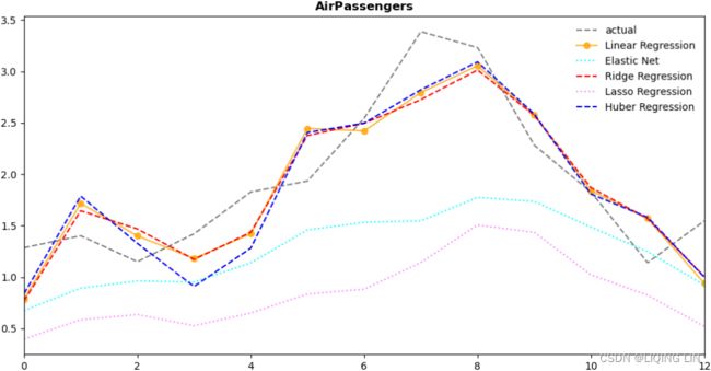

dw_results[cols].sort_values('MASE')

cols = ['yhat', 'resid', 'actual', 'Model Name']
plot_resultMix(cols, dw_results, 'Daily Temperature')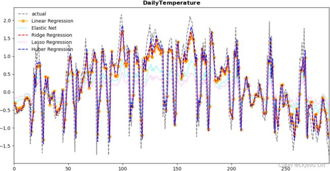

Regression Coefficients and Feature Selection

Let's examine this concept and see whether one feature is sufficient for the energy consumption dataset. Retrain the models using only the 10th feature, as in the following:

energy_10_1[-11:]

en_10 = energy_10_1[ ['y', 'x_10'] ] # at time t, y=x_t, X=x_t-1
train_en10, test_en10 = split_data( en_10, test_split=0.10 )

scaler_en10 = Standardize()
train_en10_s, test_en10_s = scaler_en10.fit_transform( train_en10, test_en10 )

train_en10_s

# regressors = { 'Linear Regression': LinearRegression(fit_intercept=False),
#                # alpha:Constant that multiplies the penalty terms. and l1_ratio=0.5 Ridge + Lasso
#                'Elastic Net': ElasticNet(alpha=0.5, fit_intercept=False), # False, the data is assumed to be already centered
#                'Ridge Regression': Ridge(alpha=0.5, fit_intercept=False),
#                'Lasso Regression': Lasso(alpha=0.5, fit_intercept=False),
#                'Huber Regression': HuberRegressor(fit_intercept=False)
#              }
en_10_results = train_different_models(train_en10_s, test_en10_s, regressors)

pd.DataFrame(en_10_results)

cols = ['Model Name', 'RMSE', 'MAPE', 'MASE']
en_10_results = pd.DataFrame(en_10_results)
en_10_results[cols].sort_values('MASE')

different number of lag variables(as features) but with the same number of instances

$\large {\color{Blue} \approx}$
If you rank the models by the scores and plot the results, you will notice that the performance from using just one feature ( $\large x_{10}$ == $\large x_{t-1}$ ) produces similar results obtained from using all 10 features ( $\large x_{1}$ , $\large x_{2}$ , … , $\large x_{10}$ )==( $\large x_{t-10}$ , $\large x_{t-9}$ , … , $\large x_{t-1}$ )
and you also notice the impact to the performance from different regularization terms used.

#########

en_1_1 = create_lagXs_y( en_cp, 1 )
en_1_1

en_1 = energy_1_1[ ['y', 'x_1'] ] # at time t, y=x_t, X=x_t-1
train_en1, test_en1 = split_data( en_1, test_split=0.10 )

scaler_en1 = Standardize()
train_en1_s, test_en1_s = scaler_en1.fit_transform( train_en1, test_en1 )

en_1_results = train_different_models(train_en1_s, test_en1_s, regressors)

cols = ['Model Name', 'RMSE', 'MAPE', 'MASE']
en_1_results = pd.DataFrame(en_1_results)
en_1_results[cols].sort_values('MASE')

different number of instances but with the same number of lag variables(as features)

obs>

train_en1_s

obs>

test_en1_s.shape, test_en10_s.shape

#########

cols = ['yhat', 'resid', 'actual', 'Model Name']
plot_resultMix(cols, en_10_results, 'Energy Consumption')

lag_window = 10 is better than lag_window = 1 or en_1_1[ ['y', 'x_1'] ] Proved!

To learn more about the different regression models available in the scikit-learn library, visit the main regression documentation here: https://scikit-learn.org/stable/supervised_learning.html.

To learn more about how different ML algorithms for time series forecasting compare, you can reference the following research paper:
Ahmed, Nesreen K., Amir F. Atiya, Neamat El Gayar, and Hisham El-Shishiny.
An Empirical Comparison of Machine Learning Models for Time Series Forecasting.
Econometric Reviews 29, no. 5–6 (August 30, 2010): 594–621.
https: //doi.org/10.1080/07474938.2010.481556 .

cols = ['Model Name', 'Model']
en_models = en_10_results.iloc[0:4][cols] # [0:4] : exclude Huber Regression
 
for row in en_models.iterrows():
    print(row[1][0])       # Model Name 
    print(row[1][1].coef_) # .intercept_ :[0.0, 0.0, 0.0, 0.0]

In the next recipe, you will explore multi-step forecasting techniques.

Multi-step forecasting using linear regression models with scikit-learn

In the One-step forecasting using linear regression models with scikit-learn recipe, you
implemented a one-step forecast; you provide a sequence of values for the past 10 periods
( $\large x_{1}$ , $\large x_{2}$ , … , $\large x_{10}$ )==( $\large x_{t-10}$ , $\large x_{t-9}$ , … , $\large x_{t-1}$ ) and the linear model will forecast the next period ( $\large x_{11} = x_{t}$ ), which is referred to as $\large Y$ . This is called one-step forecasting.

For example, in the case of energy consumption, to get a forecast for December 2021 you need to provide data for the past 10 months (February to November). This can be reasonable for monthly data, or quarterly data, but what about daily or hourly? In the daily temperature data, the current setup means you need to provide temperature values for the past 10 days to obtain a one-day forecast (just one day ahead). This may not be an efficient approach since you have to wait until the next day to observe a new value to feed to the model to get another one-day forecast.

What if you want to predict more than one future step? For example, you want three months into the future ( $\large x_{11}$ , $\large x_{12}$ , $\large x_{13}$ )==( $\large x_t$ , $\large x_{t+1}$ , $\large x_{t+2}$ ) based on a sequence of 10 months ( $\large x_{1}$ , $\large x_{2}$ , … , $\large x_{10}$ )==( $\large x_{t-10}$ , $\large x_{t-9}$ , … , $\large x_{t-1}$ ). This concept is called a multi-step forecast. In the Preparing time series data for supervised learning recipe, we referenced the paper Machine Learning Strategies for Time Series Forecasting for preparing time series data for supervised ML. The paper also discusses four strategies for multi-step forecasting, such as the Recursive strategy, the Direct strategy, DirRec (Direct-Recursive) strategy, and Multiple Output strategies.

In this recipe, you will implement a Recursive forecasting strategy. This will help you gain an idea of what a multi-step forecasting is all about. This is useful when you want to forecast further into the future beyond the out-of-sample (test) data that you have at hand.

The following illustrates the idea behind the recursive strategy. It is still based on one-step forecasts that are reused (recursively) to make the next one-step prediction, and the process continues (think of a loop) until you get all the future steps, known as future horizons, produced.

Figure 12.5 – Sliding window (five periods) with multi-step forecasts of daily temperature

At each step in Figure 12.5, you are still performing a one-step forecast.

The gray boxes represent the actual observed values, and
the black boxes represent estimated or forecasted values.

If you want to forecast into the future, let's say five periods ahead, and your actual observed data ends on 2017-01-01, you will need to provide five past periods from 2016-12-28 to 2017-01-01 to get a one-step forecast for 2017-01-02. The estimated value on 2017-01-02 is used as an input to estimate the next one-step to forecast for 2017-01-03. This recursive behavior continues until all five future steps (horizons) are estimated.

In this recipe, you will be using the models obtained from the previous One-step forecasting using linear regression models with scikit-learn recipe. A recursive multi-step strategy is used in the forecasting (prediction) phase:

1. From the previous recipe, you should have three DataFrames ( air_results, dw_results, and en_results ) that contain the results from the trained models. The following steps will use dw_results for demonstration (daily weather), you should be able to apply the same process on the remaining DataFrames (as demonstrated in the accompanying Jupyter Notebook).

air_results = train_different_models(train_air_s, test_air_s, regressors)
en_results = train_different_models(train_en_s, test_en_s, regressors)
# train_dw, test_dw = split_data( daily_temp_10_1, test_split=0.10 )
# scaler_dw = Standardize()
# train_dw_s, test_dw_s = scaler_dw.fit_transform( train_dw, test_dw )
dw_results = train_different_models(train_dw_s, test_dw_s, regressors)

air_results = pd.DataFrame(air_results)
en_results = pd.DataFrame(en_results)
dw_results = pd.DataFrame(dw_results)

dw_results

Extract the model and the model's name. Recall that there are five trained models:

models_dw = dw_results[['Model Name', 'Model']]
models_dw

2. Create the multi_step_forecast function, which consists of a for loop that makes a one-step future forecast (estimate) using the model's predict method. On each iteration or step, the estimated value is used as input to produce the next one-step estimate for another future step:

def multi_step_forecast( input_window, model, steps=10 ):
    forecast = []
    for i in range( steps ):
        one_step_pred = model.predict( np.array(input_window).reshape(1,-1) )[0]
        forecast.append( one_step_pred )
        _ = input_window.pop(0)                # input_window = np.roll(input_window, shift=-1)#left shift
        input_window.append( one_step_pred )   # input_window[-1] = one_step_pred
    return np.array( forecast )

In the Jupyter notebook, there is another version of the multi_step_forecast function that takes a NumPy array instead of a Python list. In NumPy, you can use the roll function as opposed to the pop and append methods used here. Both implementations work the same way.

3. Capture the last row from test_dw_s DataFrame. This represents the last 10 observations. Recall that the DataFrame was created using a 10-period sliding window, and the last row represents observations from 2016-12-23 to 2017-01-01:

dw_cp[-11:]

test_dw.iloc[-10:]

test_dw_s.iloc[-10:]

test_dw_s.iloc[[-10]] # last two rows: test_dw_s.iloc[[-2,-1]]

test_dw_s.iloc[-10] # ==test_dw_s.iloc[(-10,)]

### y=-1.020165 : 2016-12-23

dw_ms = test_dw_s.drop( columns=['y'] ).iloc[-10].tolist()
dw_ms

Daily Temperature

4. Loop through the models and pass the dw_ms list, the model, and the number of future steps (for example, 10 future steps) to the multi_step_forecast function:

The predicted values are stored in the frcst_dw dictionary. The values have been inversely scaled to their original scale using the inverse_y method.

frcst_dw = {}
models = dw_results[ ['Model Name', 'Model'] ]
dw_ms = test_dw_s.drop( columns=['y'] ).iloc[-10].tolist()

# scaler_dw = Standardize()
# train_dw_s, test_dw_s = scaler_dw.fit_transform( train_dw, test_dw ) # mu and std from train_dw

for r in models.iterrows():
    # r[0] : the dataframe index
    # r[1] : 'Model name', 'Model'
    pred = multi_step_forecast( dw_ms, steps=10, model=r[1]['Model'] )
    pred = scaler_dw.inverse_y( pred )

    frcst_dw[ r[1]['Model Name'] ] = pred

frcst_dw

5. Create a plot to compare actuals versus predicted for the daily temperature data:

for name, pred in frcst_dw.items():
    actual = dw_cp.iloc[-10:]
    
    ax = actual.plot( style='k-.', figsize=(10,4) )
    pd.Series( pred, index = dw_cp.index[-10:] ).plot( style='b--o', ax=ax )
    
    plt.title( r'Multi-Step Forecasting with $\bf{}$'.format(name) )
    plt.legend( ['actual', 'forecast'] )
    plt.show()

The preceding code should produce five plots; a plot for each model. The following shows the output from the first model: Linear Regression. Figure 12.6 – 10-day forecast using a recursive multi-step forecast
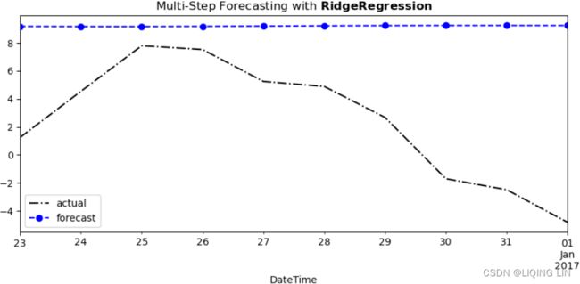
Figure 12.6 – 10-day forecast using a recursive multi-step forecast One problem with the recursive strategy is that as you go further into the future, you are exclusively relying on the estimated values and any associated estimation errors. This can cause an accumulated effect of these errors as you progress further into the future, making the forecast highly biased.

color_list = ['cyan', 'red', 'black', 'orange', 'blue']
ls_list = [ ':',       ':',     ':',    ':',     ':']
marker_list=['*',       'o',     'x',     's',   '.']
marker_size=[8,         20,       20,      12,   10]

actual = dw_cp.iloc[-10:]
ax = actual.plot( style='m--.', figsize=(10,4), legend=True )

for idx, (name, pred) in enumerate( frcst_dw.items() ):
    pd.Series( pred, index = dw_cp.index[-10:] ).plot( color=color_list[idx],
                                                       linestyle=ls_list[idx],
                                                       marker=marker_list[idx],
                                                       markersize=marker_size[idx],
                                                       #markerfacecolor='white',
                                                       markeredgecolor=color_list[idx],
                                                       alpha=1,
                                                       label=name,
                                                       legend=True,
                                                       ax=ax 
                                                     )
plt.title( r'Multi-Step Forecasting with $\bf{}$ dataset'.format('Daily Temperature') )
plt.show()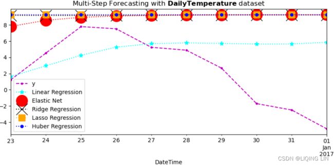

Air Passengers

air_cp[-11:]

test_air[-10:]

test_air_s[-10:]

frcst_air = {}
models = air_results[ ['Model Name', 'Model'] ]
air_ms = test_air_s.drop( columns=['y'] ).iloc[-10].tolist()

for r in models.iterrows():
    pred = multi_step_forecast( air_ms, steps=10, model=r[1]['Model'] )
    pred = scaler_air.inverse_y( pred )
    # r[0] : the dataframe index
    # r[1] : 'Model name', 'Model'
    frcst_air[ r[1]['Model Name'] ] = pred

frcst_air

color_list = ['cyan', 'red', 'black', 'orange', 'blue']
ls_list = [ ':',       ':',     ':',    ':',     ':']
marker_list=['*',       'o',     'x',     's',   '.']
marker_size=[8,         20,       20,      12,   10]

actual = air_cp.iloc[-10:]
ax = actual.plot( style='m--.', figsize=(10,4), legend=True )

for idx, (name, pred) in enumerate( frcst_air.items() ):
    pd.Series( pred, index = air_cp.index[-10:] ).plot( color=color_list[idx],
                                                       linestyle=ls_list[idx],
                                                       marker=marker_list[idx],
                                                       markersize=marker_size[idx],
                                                       #markerfacecolor='white',
                                                       markeredgecolor=color_list[idx],
                                                       alpha=1,
                                                       label=name,
                                                       legend=True,
                                                       ax=ax 
                                                     )
plt.title( r'Multi-Step Forecasting with $\bf{}$ dataset'.format('Air Passengers') )
plt.show()

Energy Consumption

frcst_en = {}
models = en_results[ ['Model Name', 'Model'] ]
en_ms = test_en_s.drop( columns=['y'] ).iloc[-10].tolist()

for r in models.iterrows():
    pred = multi_step_forecast( en_ms, steps=10, model=r[1]['Model'] )
    pred = scaler_en.inverse_y( pred )
    # r[0] : the dataframe index
    # r[1] : 'Model name', 'Model'
    frcst_en[ r[1]['Model Name'] ] = pred

frcst_en

color_list = ['cyan', 'red', 'black', 'orange', 'blue']
ls_list = [ ':',       ':',     ':',    ':',     ':']
marker_list=['*',       'o',     'x',     's',   '.']
marker_size=[8,         20,       20,      12,   10]

actual = en_cp.iloc[-10:]
ax = actual.plot( style='m--.', figsize=(10,4), legend=True )

for idx, (name, pred) in enumerate( frcst_en.items() ):
    pd.Series( pred, index = en_cp.index[-10:] ).plot( color=color_list[idx],
                                                       linestyle=ls_list[idx],
                                                       marker=marker_list[idx],
                                                       markersize=marker_size[idx],
                                                       #markerfacecolor='white',
                                                       markeredgecolor=color_list[idx],
                                                       alpha=1,
                                                       label=name,
                                                       legend=True,
                                                       ax=ax 
                                                     )
plt.title( r'Multi-Step Forecasting with $\bf{}$ dataset'.format('Energy Consumption') )
plt.show()

One problem with the recursive strategy is that as you go further into the future, you are exclusively relying on the estimated values and any associated estimation errors. This can cause an accumulated effect of these errors as you progress further into the future, making the forecast highly biased.

Multi-step forecasting is useful in situations that require more than one step forecast into the future. You implemented a recursive strategy to produce a multi-step forecast, which is essentially a one-step forecast repeated as many times as the number of future steps required. At each iteration, the prediction from one step is used as an input in the next step to make another one-step prediction. One of the drawbacks is that the model is using estimated values that can contain prediction errors to make more predictions.

To illustrate this, the following shows an example of extending the forecast to 20 steps (beyond the actual observations available) and you can observe how these errors accumulate.

frcst_dw = {}
models = dw_results[ ['Model Name', 'Model'] ]
dw_ms = test_dw_s.drop( columns=['y'] ).iloc[-10].tolist()

# scaler_dw = Standardize()
# train_dw_s, test_dw_s = scaler_dw.fit_transform( train_dw, test_dw ) # mu and std from train_dw

for r in models.iterrows():
    # r[0] : the dataframe index
    # r[1] : 'Model name', 'Model'
    pred = multi_step_forecast( dw_ms, steps=20, model=r[1]['Model'] )
    pred = scaler_dw.inverse_y( pred )

    frcst_dw[ r[1]['Model Name'] ] = pred

frcst_dw

import datetime

color_list = ['k', 'red', 'black', 'orange', 'blue']
ls_list = [ ':',       ':',     ':',    ':',     ':']
marker_list=['*',       'o',     'x',     's',   '.']
marker_size=[8,         20,       20,      12,   10]

actual = dw_cp.iloc[-10:]
ax = actual.plot( style='m--.', figsize=(10,4), legend=True )

datetimeindex_list = pd.date_range( dw_cp.index[-10], periods=20, freq='D')

for idx, (name, pred) in enumerate( frcst_dw.items() ):
    pd.Series( pred, index = datetimeindex_list ).plot( color=color_list[idx],
                                                       linestyle=ls_list[idx],
                                                       marker=marker_list[idx],
                                                       markersize=marker_size[idx],
                                                       #markerfacecolor='white',
                                                       markeredgecolor=color_list[idx],
                                                       alpha=1,
                                                       label=name,
                                                       legend=True,
                                                       ax=ax 
                                                     )
plt.title( r'Multi-Step Forecasting with $\bf{}$ dataset'.format('Daily Temperature') )
plt.show()

Figure 12.7 – Example of using a recursive strategy for a longer future horizon

A second approach is the direct strategy, which creates multiple models for each future step. Each model produces a one-step forecast, but they act independently. This can cause a maintenance issue; for example, to produce a 10-day forecast, you will have 10 models. Additionally, this independence is a lost opportunity to capture dependencies that would occur from one prediction to another. The direct strategy can suffer from high variance.

The third approach, the DirRec strategy, is a hybrid of direct and recursive and a way to mitigate their individual shortcomings. In the next section, you will see a fourth approach, the multiple output strategy.

In the Forecasting using non-linear models with sktime recipe, you will explore a simpler approach to implementing different multi-step strategies.

In the Multiple output strategy, you will create a similar sliding window function as you did with the create_lagXs_y function. However, the new function will also take an output window. For example, you will

provide a 10-sliding window for input and a 10-sliding window for output and
the resulting DataFrame will contain ( $\large x_1$ , $\large x_2$ , … , $\large x_{10}$ ) for the independent variables (features) and ( $\large Y_1$ , $\large Y_2$ , … , $\large Y_{10}$ ) for the target variables.
This is a one-shot approach一次性方法 in which you provide a sequence as input and get a sequence as output.

The multiple_output function takes a window_in parameter for the number of features to be generated, and a window_out parameter for the number of target variables to be generated:

def multiple_output( df, window_in, window_out ):
    d = df.values
    X_xs = []
    Y_ys = []
    n = len(df)
    idx = df.index[:-window_in]
    print( len(idx) )
    
    for start in range( n-window_in ):
        end = start + window_in
        out = end + window_out
        X_xs.append( d[start:end].ravel() )
        Y_ys.append( d[end:out].ravel() )
        
    cols_x = [ f'x_{i}' 
               for i in range(1, window_in+1) 
             ]
    cols_y = [ f'y_{i}' 
               for i in range(1, window_out+1)
             ]
    
    df_xs = pd.DataFrame( X_xs, index=idx, columns=cols_x )
    df_y = pd.DataFrame( Y_ys, index=idx, columns=cols_y )
    return pd.concat( [df_xs, df_y], axis=1 ).dropna()

The following is an example of using the multiple_output function to produce a sequence of 10 as input features and a sequence of 10 as target variables:

win_in, win_out=10, 10
dw_mo = multiple_output( dw_cp, win_in, win_out )
dw_mo.columns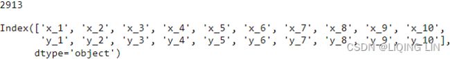

Train a linear regression model on this new dataset. Follow a similar process for splitting and scaling the data as in the previous recipe:

train_dw, test_dw = split_data( dw_mo, test_split=0.10 )
scaler_dw = Standardize()
train_dw_s, test_dw_s = scaler_dw.fit_transform( train_dw, test_dw )

test_dw[-20:]

y1 ==> 2016-12-04

test_dw_s[-20:]

y1 ==> 2016-12-04

Extract X_train, y_train, X_test, y_test:

X_train, y_train = train_dw_s.iloc[:, :win_in], train_dw_s.iloc[:, win_out:]
X_test, y_test = test_dw_s.iloc[:, :win_in], test_dw_s.iloc[:, win_out:]
X_test[-20:]

y_test[-20:]

2016-11-24 : y1 ==> 2016-12-04

Now, you can fit the model and then make a prediction:

lr = LinearRegression()
lr.fit(X_train, y_train)

mo_pred = lr.predict(X_test)[-1]
mo_pred

Create a plot to compare the forecast against the out-of-sample or test data:

mo_pred = scaler_dw.inverse_y( lr.predict(X_test)[-1] )
 # OR # pd.date_range( X_test.index[-1], periods=20, freq='D')
dates = pd.date_range('2016-12-13', freq='D', periods=20 )
dates

last_10input_date, last_10output_date = dates[:win_in], dates[win_out:]
last_10output_date

#         actual last 20 values
pd.Series( test_dw.iloc[-1].values, index=dates).plot(style='k--', 
                                                      alpha=0.5,
                                                      figsize=(10,4)
                                                     )
#        forcast last 10 values
pd.Series( mo_pred, index=last_10output_date).plot(style='k-o')
plt.title('Multiple Output for Multi-Step Forecasting with Linear Regression')
plt.legend(['Actual', 'Forecast'])
plt.show()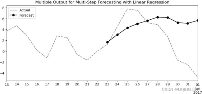

Figure 12.8 – Daily temperature 10-day forecast using the multiple output strategy

Compare the performance in Figure 12.8 with Figure 12.6.
Figure 12.6 – 10-day forecast using a recursive multi-step forecast

To learn more about multi-step forecasting, you can refer to Machine Learning Strategies for Time Series Forecasting. Lecture Notes in Business Information Processing. Berlin, Heidelberg: Springer Berlin Heidelberg. https: //doi.org/10.1007/978-3-642-36318-4_3.

Forecasting using non-linear models with sktime

In the previous recipes, you had to prepare the time series data to make it suitable for supervised ML. This is because scikit-learn ( sklearn ) is a general ML library and not specific for time series forecasting. This is where sktime is positioned to fill in the gap as a unified machine learning framework for time series. In this recipe, you will explore how to create a ML pipeline that prepares any time series data and can use algorithms from a standard ML library such as sklearn.

In Chapter 13, Deep Learning for Time Series Forecasting, you will explore other non-linear models, such as Recurrent Neural Networks. In this recipe, you will explore different algorithms that can capture non-linear relationships such as K-Nearest Neighbors Regression.

You will train multiple regressors (linear and non-linear) from sklearn . The recipe will cover data preparation, model training, forecasting, and comparing performance between the models. You will create a pipeline using the TransforemdTargetForecaster class from sktime.

You will be working with the energy consumption dataset that was loaded earlier in the Technical requirements section.

import sktime
sktime.__version__

Note in the following the energy consumption data is used for demonstration. You should be able to apply the same process on the other two datasets:

1. Make a copy of the energy DataFrame for this recipe:

df_en = energy.copy() # default deep=True
df_en

df_en.index.year.unique()

df_en.plot( title=r'$\bfMonthly$ Energy Consumption',
            figsize=(10,6)
          )
plt.show()

The Augmented Dickey-Fuller test can be used to test for a unit root in a univariate process in the presence of serial correlation.

This determines the presence of a unit root in time series.

If a unit root is present, the time series is not stationary.
The null hypothesis $\small H_0$ of this test is that the series has a unit root.
If we reject the null hypothesis, this means that we don't find a unit root.
If we fail to reject the null hypothesis, we can say that the time series is non-stationary

from statsmodels.tsa.api import seasonal_decompose, adfuller

adfuller( df_en )

(-1.4497331132437548, # The test statistic.

0.5582151234544153, # MacKinnon’s approximate p-value based on MacKinnon

12, # The number of lags used.

575, # The number of observations used for the ADF regression and
calculation of the critical values.

{'1%': -3.4417738839904657, # Critical values for the test statistic at the 1 %
'5%': -2.8665796253604015, # Critical values for the test statistic at the 5 %
(95% confidence level)
'10%': -2.569453974291115}, # Critical values for the test statistic at the 10 %
6916.6482184861825 # The maximized information criterion if autolag is not None.
(default autolag='AIC', $\large AIC = 2k - 2ln(\hat{L})$ )
)

The ADF test statistic value is more than the all critical values, and the p-value is more than 0.05. With these, we cannot reject the null hypothesis $\large H_0$ that there is a unit root and consider that our data is non-stationary.

The Akaike Information Criterion (AIC) is a metric that aims to find a balance between a model's maximum likelihood and a model's simplicity. Overly complex models can sometimes overfit, meaning they can look like they learned but once they are presented with unseen data, they perform poorly. The AIC score penalizes as the number of parameters increases since they increase complexity:

k is the total number of parameters learned or estimated by the model and initial states that have been estimated (including the residual variance).. For example, in multiple linear regression, the estimated parameters are the intercept, the slope parameters, and the constant variance of the errors; thus ,
Here, 2k is considered the penalty term.ts10_Univariate TS模型_circle mark pAcf_ETS_unpack product_darts_bokeh band interval_ljungbox_AIC_BIC_LIQING LIN的博客-CSDN博客
$\large \hat{L}$ is the maximized value of the likelihood function of the model M. i.e. , where are the parameter values that maximize the likelihood function, = the observed data;09_2_Semi监督(kmeans+log_reg)_propagate_EM_np.percentile_DBSCAN+knn_Spectral_BayesianGaussi_Likelihood_LIQING LIN的博客-CSDN博客_xmoon.best
if you don’t know θ, and instead if you have observed a single instance x=2.5 (the vertical line in the upper-left plot)? In this case, you get the likelihood function ℒ(θ|x=2.5)=f(x=2.5; θ), represented in the upper-right plot.

plt.rcParams['figure.figsize'] = (10,8)

decomposed_en = seasonal_decompose( df_en, model='additive', )
fig=decomposed_en.plot()

axs = fig.get_axes()
axs[3].clear()
axs[3].plot(decomposed_en.resid)
axs[3].axhline(y=0, color='k', linestyle='--')
axs[3].set_ylabel('Resid')

plt.show()

Monthly data ==> seasonal periods=12

decomposed_add = seasonal_decompose( df_en, period=12, model='additive')
decomposed_mul = seasonal_decompose( df_en, period=12, model='multiplicative')
                              ###########  
fig, axes = plt.subplots(4,1, sharex=True, figsize=(12,12))
 
comps = ["observed","trend", "seasonal", "resid"]
ylabels = ["Data", "Trend", "Seasonal", "Resid"]
colors = ["blue","k"]
alphas=[1, 1]
linewidths=[1,1]
 
for i, decomposed in enumerate( [decomposed_add, decomposed_mul] ):
    for idx, ax in enumerate(axes):
        
        series = getattr(decomposed, comps[idx])
        
        if i == 0:                       
            ax.set_ylabel('Additive '+ ylabels[idx], fontsize = 12, color=colors[i])
        else:
            ax=ax.twinx()
            ax.set_ylabel('Multiplicative '+ ylabels[idx], fontsize = 12, 
                           rotation=270, labelpad=12, color=colors[i])
            
#         if comps[idx] == "resid":
#             ax.plot(series, color=colors[i], marker='o', markersize=5, 
#                     linestyle="none", alpha=alphas[i])
#             # nobs = decomposed.observed.shape[0]
#             # xlim = decomposed.observed.index[0], decomposed.observed.index[nobs - 1]
#             # ax.plot(xlim, (0, 0), color=colors[i], zorder=-3)
            
#         else:
#             ax.plot(series, color=colors[i], alpha=alphas[i], 
#                     linewidth=linewidths[i])
        ax.plot(series, color=colors[i], alpha=alphas[i], linewidth=linewidths[i])
        if comps[idx] == "resid":
            ax.axhline(y=0, color=colors[i], linestyle='--')

            
plt.show()

better to use 'additive' model

2. You will need to split the data into training and test sets using the split_data function created earlier:

# def split_data( df, test_split=0.15 ):
#     n = int( len(df) * test_split )
#     train, test = df[:-n], df[-n:]
#     return train, test

train_en, test_en = split_data(df_en)
train_en.shape, test_en.shape

3. The sktime library uses a similar ML framework as scikit-learn, such as the use of the fit method for training a model and the predict method to make predictions. You will explore five different regressors from sklearn:

Linear Regression,
Random Forest Regressor,
Gradient Boosting Regressor,
Extra Tree Regressor, and
KNN Regressor.

You will include a Naive Forecaster with a mean strategy. The Naive Forecaster will be the baseline model to compare how the other regressors perform.

from sklearn.linear_model import LinearRegression
from sklearn.ensemble import (RandomForestRegressor,
                              GradientBoostingRegressor,
                              ExtraTreesRegressor
                             )
from sklearn.neighbors import KNeighborsRegressor

from sktime.forecasting.all import ( NaiveForecaster,
                                     Deseasonalizer, Detrender, 
                                     temporal_train_test_split,
                                     mean_absolute_percentage_error as mape,
                                     mean_squared_percentage_error as mspe,
                                     mean_squared_error as mse,
                                     ForecastingHorizon,
                                     TransformedTargetForecaster,
                                     PolynomialTrendForecaster
                                   )
from sktime.forecasting.compose import make_reduction

############# Forecasting with sktime — sktime documentation

1. Basic forecasting workflows

Step 1 - Preparation of the data

from sktime.datasets import load_airline
from sktime.utils.plotting import plot_series

# in the example, we use the airline data set.
y = load_airline()
plot_series(y)

ForecastingHorizon

class ForecastingHorizon(values: Optional[Union[int, 
                                                list, 
                                                numpy.ndarray, 
                                                pandas.core.indexes.base.Index
                                               ]
                                         ] = None, 
                         is_relative: Optional[bool] = None, 
                         freq=None
                        )

Forecasting horizon.

The ForecastingHorizon object takes absolute indices as input, but considers the input absolute or relative depending on the is_relative flag.

ForecastingHorizon will

automatically assume a relative horizon if temporal difference types时间差异类型 from pandas are passed;
if value types from pandas are passed, it will assume an absolute horizon.

Parameters

values pd.Index, pd.TimedeltaIndex, np.array, list, pd.Timedelta, or int

Values of forecasting horizon

is_relative bool, optional (default=None)

If True, a relative ForecastingHorizon is created:

values are relative to end of training series.
If False, an absolute ForecastingHorizon is created:

values are absolute.
if None, the flag is determined automatically:

relative, if values are of supported relative index type absolute, if not relative and values of supported absolute index type

freq str, pd.Index, pandas offset, or sktime forecaster, optional (default=None)

object carrying frequency information on values ignored unless values is without inferrable freq

Attributes

freq

Frequency attribute.

is_relative

Whether forecasting horizon is relative to the end of the training series.

Step 2 - Specifying the forecasting horizon

Now we need to specify the forecasting horizon and pass that to our forecasting algorithm.

There are two main ways:

Using a numpy.array of integers. This assumes either integer index or periodic index (PeriodIndex) in the time series; the integer indicates the number of time points or periods ahead we want to make a forecast for. E.g., 1 means forecast the next period, 2 the second next period, and so on.
```
fh = np.arange(1, 37)
fh
```
This will ask for monthly predictions for the next three years, since the original series period is 1 month. In another example, to predict only the second and fifth month ahead, one could write:
```
import numpy as np
fh = np.array([2, 5])  # 2nd and 5th step ahead
```
Using a ForecastingHorizon object. This can be used to define forecast horizons, using any supported index type as an argument. No periodic index is assumed.

from sktime.forecasting.base import ForecastingHorizon

fh = ForecastingHorizon( pd.PeriodIndex( pd.date_range("1961-01", 
                                                       periods=36, 
                                                       freq="M"
                                                      )
                                       ), 
                         is_relative=False
                       )
fh

ForecastingHorizon-s can be converted from relative to absolute and back via the to_relative and to_absolute methods. Both of these conversions require a compatible cutoff to be passed:

cutoff = pd.Period( "1960-12", freq="M" )
cutoff

# Cut-off = “present time” state of forecaster.

fh.to_relative(cutoff)

fh.to_relative(cutoff).to_absolute(cutoff) # or fh.to_absolute(cutoff)

NaiveForecaster

class NaiveForecaster(strategy='last', window_length=None, sp=1)

Forecast based on naive assumptions about past trends continuing.

NaiveForecaster is a forecaster that makes forecasts using simple strategies. Two out of three strategies are robust against NaNs对 NaN 具有鲁棒性. The NaiveForecaster can also be used for multivariate data and it then applies internally the ColumnEnsembleForecaster, so each column is forecasted with the same strategy.

Internally, this forecaster does the following: - obtains the so-called “last window”, a 1D array that denotes the

most recent time window that the forecaster is allowed to use

reshapes the last window into a 2D array according to the given seasonal periodicity (prepended with NaN values to make it fit前面加上 NaN 值以使其适合);
make a prediction for each column, using the given strategy: -
“last”: last non-NaN row “mean”: np.nanmean over rows
tile the predictions平铺预测 using the seasonal periodicity

To compute prediction quantiles为了计算预测分位数,

we first estimate the standard error of prediction residuals under the assumption of uncorrelated residuals.
The forecast variance is then computed by multiplying the residual variance by a constant. This constant is a small-sample bias adjustment and each method (mean, last, drift) have different formulas for computing the constant. These formulas can be found in the Forecasting: Principles and Practice textbook (Table 5.2) [1].
Lastly, under the assumption that residuals follow a normal distribution, we use the forecast variance and z-scores of a normal distribution to estimate the prediction quantiles.

Parameters

strategy {“last”, “mean”, “drift”}, default=”last”

Strategy used to make forecasts:

“last”: (robust against NaN values 对 NaN 值具有鲁棒性)

forecast the last value in the training series when sp is 1.
When sp is not 1, last value of each season in the last window will be forecasted for each season.将为每个季节预测最后一个窗口中每个季节的最后一个值。
“mean”: (robust against NaN values)

forecast the mean of last window of training series when sp is 1.
When sp is not 1, mean of all values in a season from last window will be forecasted for each season.将为每个季节预测最后一个窗口的一个季节中所有值的平均值
“drift”: (not robust against NaN values)

forecast by fitting a line between the first and last point of the window and extrapolating it into the future将其外推到未来来进行预测.

sp int, or None, default=1

Seasonal periodicity to use in the seasonal forecasting. None=1.

window_length int or None, default=None

Window length to use in the mean strategy. If None, entire training series will be used.

Attributes

cutoff

Cut-off = “present time” state of forecaster.

Forecasting horizon that was passed.

is_fitted

Whether fit has been called.

Step 3 - Specifying the forecasting algorithm

To make forecasts, a forecasting algorithm needs to be specified. This is done using a scikit-learn-like interface. Most importantly, all sktime forecasters follow the same interface, so the preceding and remaining steps are the same, no matter which forecaster is being chosen.

For this example, we choose the naive forecasting method of predicting the last seen value. More complex specifications are possible, using pipeline and reduction construction syntax; this will be covered later in Section 2.

from sktime.forecasting.naive import NaiveForecaster

# step 2: specifying forecasting horizon
fh = np.arange(1, 37)

# step 3: specifying the forecasting algorithm
forecaster = NaiveForecaster(strategy="last", sp=12)

predicting the latest value observed in the same month

Step 4 - Fitting the forecaster to the seen data

Now the forecaster needs to be fitted to the seen data:

forecaster.fit(y) #### ####

Step 5 - Requesting forecasts

Finally, we request forecasts for the specified forecasting horizon. This needs to be done after fitting the forecaster:

y_pred = forecaster.predict(fh) #### ####

# plotting predictions and past data
plot_series(y, y_pred, labels=["y", "y_pred"])

1.2.2 Forecasters that require the horizon already in `fit`

Some forecasters need the forecasting horizon provided already in fit. Such forecasters will produce informative error messages when it is not passed in fit. All forecaster will remember the horizon when already passed in fit for prediction. The modified workflow to allow for such forecasters in addition is as follows:

# step 1: data specification
y = load_airline()

# step 2: specifying forecasting horizon
fh = np.arange(1, 37)

# step 3: specifying the forecasting algorithm
forecaster = NaiveForecaster(strategy="last", sp=12)

# step 4: fitting the forecaster
forecaster.fit(y, fh=fh) #### ####

# step 5: querying predictions
y_pred = forecaster.predict() #### ####

# plotting predictions and past data
plot_series(y, y_pred, labels=["y", "y_pred"])

1.2.3 Forecasters that can make use of exogeneous data

Many forecasters can make use of Exogeneous time series, i.e., other time series that are not forecast, but are useful for forecasting y. Exogeneous time series are always passed as an X argument, in fit, predict, and other methods (see below). Exogeneous time series should always be passed as pandas.DataFrames. Most forecasters that can deal with exogeneous time series will assume that

the time indices of X passed to fit are a super-set of the time indices in y passed to fit;
and that the time indices of X passed to predict are a super-set of time indices in fh,
although this is not a general interface restriction.
Forecasters that do not make use of exogeneous time series still accept the argument (and do not use it internally).

The general workflow for passing exogeneous data is as follows:

# step 1: data specification
y = load_airline()
# we create some dummy exogeneous data
X = pd.DataFrame(index=y.index)

X

<==

# step 2: specifying forecasting horizon
fh = np.arange(1, 37)

# step 3: specifying the forecasting algorithm
forecaster = NaiveForecaster(strategy="last", sp=12)

# step 4: fitting the forecaster
forecaster.fit(y, X=X, fh=fh)     ####### forecasting horizon

# step 5: querying predictions
y_pred = forecaster.predict(X=X)  #######

# plotting predictions and past data
plot_series(y, y_pred, labels=["y", "y_pred"])

NOTE: as in workflows 1.2.1 and 1.2.2, some forecasters that use exogeneous variables may also require the forecasting horizon only in predict. Such forecasters may also be called with steps 4 and 5 being

# step 1: data specification
y = load_airline()
# we create some dummy exogeneous data
X = pd.DataFrame(index=y.index)

# step 2: specifying forecasting horizon
fh = np.arange(1, 37)

# step 3: specifying the forecasting algorithm
forecaster = NaiveForecaster(strategy="last", sp=12)

# step 4: fitting the forecaster
forecaster.fit(y, X=X)                 ##############

# step 5: querying predictions
y_pred = forecaster.predict(fh=fh, X=X)##############forecasting horizon

# plotting predictions and past data
plot_series(y, y_pred, labels=["y", "y_pred"])

1.2.4. Multivariate forecasting

All forecasters in sktime support multivariate forecasts - some forecasters are “genuine” multivariate, all others “apply by column”.

Below is an example of the general multivariate forecasting workflow, using the VAR (vector auto-regression) forecaster on the Longley dataset from sktime.datasets. The workflow is the same as in the univariate forecasters, but the input has more than one variables (columns).

from sktime.datasets import load_longley
from sktime.forecasting.var import VAR

_, y = load_longley()

_

Time Series / Date functionality — pandas 0.13.1 documentation

A	year end frequency

B	business day frequency

S	secondly frequency

(B)A(S)-DEC

annual frequency, anchored end of December. Same as ‘A’

The input to the multivariate forecaster y is a pandas.DataFrame where each column is a variable.

from mpl_toolkits.mplot3d import Axes3D
import matplotlib.pyplot as plt
from matplotlib.dates import DateFormatter


y = y.drop( columns=["UNEMP", "ARMED", "POP"]) 

forecaster = VAR()
forecaster.fit(y, fh=[1, 2, 3])

y_pred = forecaster.predict()

# plotting predictions and past data

fig = plt.figure()
ax = fig.add_subplot( projection="3d")

ax.plot( y.index.year, #.tolist(), 
         y.GNPDEFL, 
         y.GNP , 
         marker='.'
       )
ax.plot( y_pred.index.year,#y.index.to_timestamp(freq='A-DEC')
         y_pred.GNPDEFL, 
         y_pred.GNP, 
         marker='.' 
       )
ax.legend(["y", "y_pred"])
#plt.setp( ax.get_xticklabels(), rotation=30, horizontalalignment='right' )

plt.show()

Forecasting with sktime — sktime documentation

Deseasonalizer

class Deseasonalizer(sp=1, model='additive')

Remove seasonal components from a time series.

Fit computes seasonal components and stores them in seasonal_.

Transform aligns seasonal components stored in _seasonal with the time index of the passed series and then substracts them (“additive” model $\small y_t = S_t + T_t + R_t$ ) from the passed series or divides the passed series by them (“multiplicative” model $\small y_t = S_t \times T_t \times R_t$ ).

Parameters

sp : int, default=1

Seasonal periodicity.

model {“additive”, “multiplicative”}, default=”additive”

Model to use for estimating seasonal component.
The additive decomposition is the most appropriate if the magnitude of the seasonal fluctuations, or the variation around the trend-cycle, does not vary with the level of the time series. When the variation in the seasonal pattern, or the variation around the trend-cycle, appears to be proportional to the level of the time series, then a multiplicative decomposition is more appropriate. Multiplicative decompositions are common with economic time series.

Attributes

seasonal_ : array of length sp

Seasonal components computed in seasonal decomposition.

PolynomialTrendForecaster

If the data set is large enough and the data alternately increases and decreases数据交替增加和减少, fluctuates - go up and down, the best type of trend line is polynomial. However, keep in mind that the polynomial trend is intended to describe the current data set and calculate the values within it. It is not intended for making predictions at all. See more about the different types of trendlines you can create in Excel: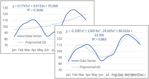

The charts above show polynomial trendlines for the same data with a degree of 2 - the minimum degree of a polynomial trendline in Excel - and 4.

The degree of the polynomial determines the maximum number of extrema - local minima or maxima of the curve:

A polynomial trendline of the second degree (also known as a Quadratic polynomial trend line : a degree of 2) can describe only one maximum or minimum (one hill or valley).
A polynomial trendline of the third degree (also known as a Cubic polynomial trend line : a degree of 3) has one or two extrema.

The maximum degree of the polynomial trendline that can be displayed in an Excel chart is 6: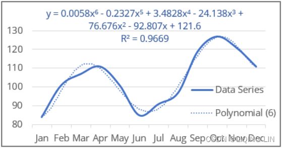

Polynomial trend equation and forecast - Microsoft Excel 365

class PolynomialTrendForecaster(regressor=None, degree=1, with_intercept=True)

Forecast time series data with a polynomial trend.

Default settings train a linear regression model with a 1st degree polynomial transformation of the feature.

Parameters

regressor estimator object, default = None

Define the regression model type. If not set, will default to sklearn.linear_model.LinearRegression

degree int, default = 1

Degree of polynomial function
A polynomial’s degree is the highest or the greatest power of a variable in a polynomial equation. The degree indicates the highest exponential power in the polynomial (ignoring the coefficients).

with_intercept bool, default=True

If true, then include a feature in which all polynomial powers are zero. (i.e. a column of ones, acts as an intercept term in a linear model)

Attributes

cutoff

Cut-off = “present time” state of forecaster.

Forecasting horizon that was passed.

is_fitted

Whether fit has been called.

Detrender

class Detrender(forecaster=None, model='additive')

Remove a trend from a series.

This transformer uses any forecaster and returns the in-sample residuals of the forecaster’s predicted values.

The Detrender works as follows: in “fit”, the forecaster is fit to the input data. in “transform”, the forecast residuals are computed and return. Depending on time indices, this can generate in-sample or out-of-sample residuals.

For example, to remove the linear trend of a time series:

forecaster = PolynomialTrendForecaster(degree=1)
transformer = Detrender(forecaster=forecaster)
yt = transformer.fit_transform(y_train)

The detrender can also be used in a pipeline for residual boosting, by first detrending and then fitting another forecaster on residuals.

Parameters

forecaster sktime forecaster, follows BaseForecaster, default = None.

The forecasting model to remove the trend with (e.g. PolynomialTrendForecaster).

If forecaster is None, PolynomialTrendForecaster(degree=1) is used.

model {“additive”, “multiplicative”}, default=”additive”

If model=”additive” the forecaster is fit to the original time series and the transform method subtracts the trend from the time series. If model=”multiplicative” the forecaster is fit to the original time series and the transform method divides the trend from the time series.

Attributes

forecaster_ Fitted forecaster

Forecaster that defines the trend in the series.

make_reduction

make_reduction(estimator, strategy='recursive', window_length=10, 
               scitype='infer', transformers=None, pooling='local'
              )

Make forecaster based on reduction to tabular or time-series regression.

During fitting, a sliding-window approach is used to first transform the time series into tabular or panel data, which is then used to fit a tabular or time-series regression estimator. During prediction, the last available data is used as input to the fitted regression estimator to generate forecasts.

Parameters

estimator an estimator instance

Either a tabular regressor from scikit-learn or a time series regressor from sktime.
The ML estimator in this recipe was the regressor (for example, LinearRegression ) that is being passed.

lr = LinearRegression()
make_reduction(lr)

strategy str, optional (default=”recursive”)

The strategy to generate forecasts. Must be one of “direct”, “recursive” or “multioutput”.
These strategies are intended for multi-step time series forecasting, similar to what is proposed and discussed in the Multi-step forecasting using linear regression models with scikit-learn recipe of this chapter. The make_reduction function makes it easy for you to explore and experiment with the different strategies. This is similar to the multi_step_forecast( input_window, model, steps=10 ) function you created earlier.

window_length int, optional (default=10)

Window length used in sliding window transformation. This is similar to the create_lagXs_y( df, lag_window ) you created earlier

scitype str, optional (default=”infer”)

Must be one of “infer”, “tabular-regressor” or “time-series-regressor”. If the scitype cannot be inferred, please specify it explicitly. See scitype.
A class or object type to denote a category of objects defined by a common interface and data scientific purpose. For example, “forecaster” or “classifier”.
For the data you are using, a DataFrame, the tabular-regressor , is selected (inferred).

transformers: list of transformers (default = None)

A suitable list of transformers that allows for using an en-bloc approach with make_reduction. This means that instead of using the raw past observations of y across the window length, suitable features will be generated directly from the past raw observations. Currently only supports WindowSummarizer (or a list of WindowSummarizers) to generate features e.g. the mean of the past 7 observations. Currently only works for RecursiveTimeSeriesRegressionForecaster.

pooling: str {“local”, “global”}, optional

Specifies whether separate models will be fit at the level of each instance (local) of if you wish to fit a single model to all instances (“global”). Currently only works for RecursiveTimeSeriesRegressionForecaster.

Returns

estimator an Estimator instance

A reduction forecaster

TransformedTargetForecaster

sktime provides a generic pipeline object for this kind of composite modelling, the TransforemedTargetForecaster. It chains an arbitrary number of transformations with a forecaster. The transformations can either be pre-processing transformations or a post-processing transformations.

class TransformedTargetForecaster(steps)

Meta-estimator for forecasting transformed time series.

Pipeline functionality to apply transformers (Deseasonalizer, Detrender and so on ) to the target series. The X data is not transformed. If you want to transform X, please use the ForecastingPipeline.

    def _get_forecaster_index(self, estimators):
        """Get the index of the first forecaster in the list."""
        return self._get_pipeline_scitypes(estimators).index("forecaster")

    @property
    def forecaster_(self):
        """Return reference to the forecaster in the pipeline.
        Returns
        -------
        sktime forecaster
            reference to unique forecaster in steps_ (without the name)
        """
        return self.steps_[self._get_forecaster_index(self.steps_)][1]

    @property
    def transformers_pre_(self):
        """Return reference to the list of pre-forecast transformers.
        Returns
        -------
        list of tuples (str, estimator) of sktime transformers
            reference to tuples that come before the unique (str, forecaster) in steps_
        """
        return self.steps_[: self._get_forecaster_index(self.steps_)]

    @property
    def transformers_post_(self):
        """Return reference to the list of post-forecast transformers.
        Returns
        -------
        list of tuples (str, estimator) of sktime transformers
            reference to tuples that come after the unique (str, forecaster) in steps_
        """
        return self.steps_[(1 + self._get_forecaster_index(self.steps_)) :]

For a list t1, t2, …, tN, f, tp1, tp2, …, tpM

where t[i] and tp[i] are transformers (t to pre-, tp to post-process), and f is an sktime forecaster, the pipeline behaves as follows:

#https://github.com/sktime/sktime/blob/v0.15.0/sktime/forecasting/compose/_pipeline.py#L634-L1088
    def _fit(self, y, X=None, fh=None):
        """Fit to training data.
        Parameters
        ----------
        y : pd.Series
            Target time series to which to fit the forecaster.
        fh : int, list or np.array, optional (default=None)
            The forecasters horizon with the steps ahead to to predict.
        X : pd.DataFrame, optional (default=None)
            Exogenous variables are ignored
        Returns
        -------
        self : returns an instance of self.
        for example :
            X = pd.DataFrame(index=y.index) # we create some dummy exogeneous data
            fh = np.arange(1, 37)           # step 2: specifying forecasting horizon
            forecaster = NaiveForecaster(strategy="last", sp=12) # forecasting algorithm
            forecaster.fit(y, X=X, fh=fh)   # step 4: fitting the forecaster
        """
        self.steps_ = self._get_estimator_tuples(self.steps, clone_ests=True)

        # transform pre
        yt = y
        for _, t in self.transformers_pre_:
            yt = t.fit_transform(X=yt, y=X)#X=yt : t[i] receiving the output of t[i-1] as X

        # fit forecaster
        f = self.forecaster_
        f.fit(y=yt, X=X, fh=fh) # with y being the output of t[N], and X=X,

        # transform post
        for _, t in self.transformers_post_:
            y = t.fit_transform(X=y, y=X)

        return self

fit(y, X, fh)

changes state by running t1.fit_transform with X=yt=y), y=X
then t2.fit_transform on X=yt from the output of t1.fit_transform, y=X, etc sequentially依次类推, with t[i] receiving the output of t[i-1] as X,
then running f.fit with y being the output of t[N], and X=X,
then running tp1.fit_transform with X=y, y=X,
then tp2.fit_transform on X=y from the output of tp1.fit_transform, etc sequentially, with tp[i] receiving the output of tp[i-1] as X,

    def _predict(self, fh=None, X=None):
        """Forecast time series at future horizon.
        Parameters
        ----------
        fh : int, list, np.array or ForecastingHorizon
            Forecasting horizon
        X : pd.DataFrame, optional (default=None)
            Exogenous time series
        Returns
        -------
        y_pred : pd.Series
            Point predictions
        """
        y_pred = self.forecaster_.predict(fh=fh, X=X)
        # inverse transform y_pred
        y_pred = self._get_inverse_transform(self.transformers_pre_, y_pred, X)

        # transform post
        for _, t in self.transformers_post_:
            y_pred = t.transform(X=y_pred, y=X)

        return y_pred

predict(X, fh)

result is of executing f.predict, with X=X, fh=fh, ==> y_pred
then running tp1.inverse_transform with X= the output of f(or X=y_pred), y=X, ==>new y_pred
then t2.inverse_transform on X= the output of t1.inverse_transform(X=y_pred), etc sequentially, with t[i] receiving the output(y_pred) of t[i-1] as X,
then running tp1.fit_transform with X= the output of t[N]s (or X=y_pred), y=X, ==> y_pred then tp2.fit_transform on X= the output of tp1.fit_transform(y_pred), etc sequentially, with tp[i] receiving the output of tp[i-1],

predict_interval(X, fh), predict_quantiles(X, fh) - as predict(X, fh),

with predict_interval or predict_quantiles substituted代替 for predict

predict_var, predict_proba - uses base class default to obtain

crude estimates粗略估计 from predict_quantiles. Recommended to replace with better custom implementations if needed.

get_params, set_params uses sklearn compatible nesting interface

if list is unnamed, names are generated as names of classes if names are non-unique, f”_{str(i)}” is appended to each name string

where i is the total count of occurrence of a non-unique string inside the list of names leading up to it (inclusive)

TransformedTargetForecaster can also be created by using the magic multiplication

on any forecaster, i.e., if my_forecaster inherits from BaseForecaster,

and my_t1, my_t2, my_tp inherit from BaseTransformer, then, for instance, my_t1 * my_t2 * my_forecaster * my_tp will result in the same object as obtained from the constructor TransformedTargetForecaster([my_t1, my_t2, my_forecaster, my_tp])

forecaster = TransformedTargetForecaster(
    [
        ("deseasonalize", Deseasonalizer(model="multiplicative", sp=12)),
        ("forecast", ARIMA()),
    ]
)

forecaster = Deseasonalizer(model="multiplicative", sp=12) * ARIMA()
forecaster

magic multiplication can also be used with (str, transformer) pairs, as long as one element in the chain is a transformer

Parameters

steps list of sktime transformers and forecasters, or

list of tuples (str, estimator) of sktime transformers or forecasters

the list must contain exactly必须恰好包含 one forecaster

these are “blueprint” transformers resp forecasters,

forecaster/transformer states do not change when fit is called

Attributes

steps_ list of tuples (str, estimator) of sktime transformers or forecasters

clones of estimators in steps which are fitted in the pipeline is always in (str, estimator) format, even if steps is just a list strings not passed in steps are replaced by unique generated strings i-th transformer in steps_ is clone of i-th in steps

forecaster_ estimator, reference to the unique forecaster in steps_

Return reference to the forecaster in the pipeline.

transformers_pre_ list of tuples (str, transformer) of sktime transformers

Return reference to the list of pre-forecast transformers.

transformers_ost_ list of tuples (str, transformer) of sktime transformers

reference to pairs in steps_ that succeed forecaster_

https://github.com/sktime/sktime/blob/v0.15.0/sktime/forecasting/compose/_pipeline.py#L634-L1088

Example 1: string/estimator pairs

pipe = TransformedTargetForecaster(steps=[
    ("imputer", Imputer(method="mean")),
    ("detrender", Detrender()),
    ("forecaster", NaiveForecaster(strategy="drift")),
])
pipe.fit(y)
y_pred = pipe.predict(fh=[1,2,3])

Example 2: without strings

pipe = TransformedTargetForecaster([
    Imputer(method="mean"),
    Detrender(),
    NaiveForecaster(strategy="drift"),
    ExponentTransformer(),
])

Example 3: using the dunder method

forecaster = NaiveForecaster(strategy="drift")
imputer = Imputer(method="mean")
pipe = imputer * Detrender() * forecaster * ExponentTransformer()

#############

Since the process for training the models is similar on all regressors, you will create a function, make_forecast , that takes in the training dataset, a regressor, the number of future horizons (steps), and a window size. The function returns a pandas Series of the predicted values.

In the make_forecast function, you will create a pipeline using the TransformedTargetForecaster class to apply a set of transformations, for example, removing trend and seasonality using the Detrender and Deseasonalizer classes, respectively. You have performed these tasks individually in ts10_Univariate TS模型_circle mark pAcf_ETS_unpack product_darts_bokeh band interval_ljungbox_AIC_BIC_LIQING LIN的博客-CSDN博客ts10_2Univariate TS模型_pAcf_bokeh_AIC_BIC_combine seasonal_decompose twinx ylabel_bold partial title_LIQING LIN的博客-CSDN博客_first-order diff, Building Univariate Time Series Models Using Statistical Methods. Here you will leverage the TransformedTargetForecaster class to chain these steps:

In this recipe, you will be able to use multiple regressors from the sklearn library by leveraging sktime. This is made possible using the TransformedTargetForecaster class and the make_reduction function. TransformedTargetForecaster allow you to create a chain of steps, a pipeline, to transform the time series. For example, three transformations were used: the Deseasonalizer class, the Detrender class, and the make_reduction function.

You can think of the make_reduction function (from sktime) as comparable to the create_lagXs_y( df, lag_window ) and the multi_step_forecast( input_window, model, steps=10 ) functions you created in earlier recipes. For example, the make_reduction function was used to prepare the time series allowing you to use any regressor from the scikit-learn library

def make_forecast( data, n_steps, regressor, window=12 ):
    fh = ForecastingHorizon( np.arange(n_steps)+1, 
                             is_relative=True # True: forecasting horizon is relative to the end of the training series
                           )
    forecaster = [ ( "deseasonalize", Deseasonalizer(sp=12, model='additive') ),
                   ( "detrend", Detrender( forecaster=PolynomialTrendForecaster(degree=1) ) )
                 ]
    
    if not isinstance( regressor, NaiveForecaster ):
        reg = ("forecaster", make_reduction( regressor,
                                             strategy='recursive', # default
                                             window_length=window,
                                             scitype='tabular-regressor'
                                           )
              )
        forecaster.append( reg )
        model = TransformedTargetForecaster( steps=forecaster ).fit( data.values )
        # TransformedTargetForecaster( forecaster ): chain transformations
        # Deseasonalizer(sp=12, model='additive') * Detrender( forecaster=PolynomialTrendForecaster(degree=1) )
    else:
        model = regressor.fit( data.values )
    
    return model.predict( fh=fh )

Notice the use of the make_reduction function in the pipeline before fitting (training) the model. This will create a reduced regression for the time series data. You will learn more on the concept of a reduced form in the How it works... section. For now, realize that make_reduction will return a RecursiveTabularRegressionForecaster class, and the default strategy parameter is recursive.

4. Create a Python dictionary for the different regressors so you can loop through and pass each one to the make_forecast function. You will append the returned predictions as a new column to the test DataFrame for easier comparison:

train, test = split_data(df_en)
test

regressors = { 'Naive Forecaster' : NaiveForecaster( strategy='mean', 
                                                     sp=12
                                                   ),
               'Linear Regression': LinearRegression(),
               'K-NN Regressor': KNeighborsRegressor(n_neighbors=5),
               'Extra Tree Regressor': ExtraTreesRegressor(),
               'Random Forest Regressor': RandomForestRegressor(),
               'Gradient Boosting Regressor': GradientBoostingRegressor()
             }

for regName, reg in regressors.items():
    print( f'training {reg} ...' )
    
    predicted = make_forecast(train, len(test), regressor=reg , window=15)
    test[regName] = pd.Series( predicted.reshape(-1), 
                               index=test.index
                             )

test

predicted

Once execution is completed, the test DataFrame should have a shape of (88, 7), indicating 88 rows and 7 columns. The last 6 columns are based on each model.

5. Plot the predictions from each regressor against the test data. To do so, loop through the results in the test DataFrame and keep in mind that the observed out-of-sample (test data) values are in the first column:

for i in test.iloc[:, 1:]: # except y
    ax = df_en[-2*len(test):].plot(style='k--', alpha=0.45, title=i, figsize=(10,5))
    
    test[i].plot(ax=ax)
    plt.legend(['Actual', i])
    plt.show()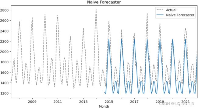

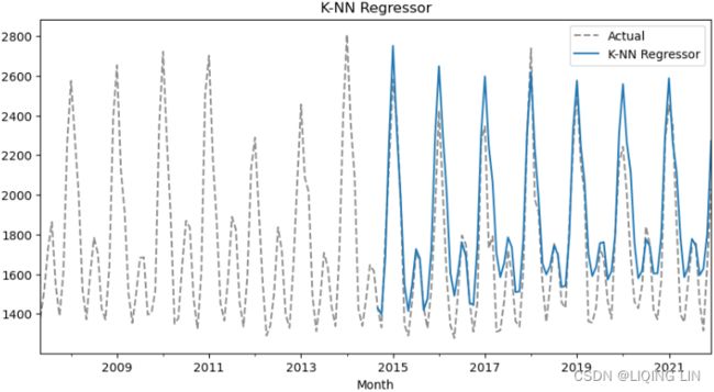
test.plot( subplots=False, figsize=(16, 12) )
plt.show()

#https://matplotlib.org/stable/tutorials/colors/colors.html
color_list = ['black', 'cyan', 'red',  '#1f77b4', 'g', 'blue', 'yellow']
facecolor_list=['black', 'cyan', 'red', '#1f77b4', 'g', 'blue', 'yellow']
ls_list = [ '-',         '--',  '--', '--', '--',   '-', '--']
lws = [         1,          2,     4,   4,    2,    2,     2]
marker_list=[None,     None,   'o',    'D',  '*',   '$R$', None]
marker_size=[0,          0,    8,       5,   10,    8, 0]
alpha_list=[0.8,        1,   0.5,    1,  0.5, 1, 1]

fig, ax = plt.subplots( figsize=(12,10) )
import matplotlib
matplotlib.rcParams.update(matplotlib.rcParamsDefault)
ax.set_facecolor('white')
for idx, (name, pred) in enumerate( test.items() ):
    pd.Series( pred, index = test.index ).plot( color=color_list[idx],
                                                       linestyle=ls_list[idx],
                                                       linewidth=lws[idx],
                                                       marker=marker_list[idx],
                                                       markersize=marker_size[idx],
                                                       markerfacecolor=facecolor_list[idx],
                                                       markeredgecolor=color_list[idx],
                                                       alpha=alpha_list[idx],
                                                       label=test.columns[idx],
                                                       legend=True,
                                                       ax=ax 
                                                     )
plt.title( r'Multi-Step Forecasting with $\bf{}$ dataset'.format('Energy Consumption') )
plt.show()

import plotly.graph_objects as go

def plotly_predMix( results, data_name, x_title='', y_title='' ):

    # https://stackoverflow.com/questions/59953431/how-to-change-plotly-figure-size
    layout=go.Layout(width=1000, height=900, 
                     title=f'{data_name}',
                     title_x=0.5, title_y=0.9,
                     xaxis=dict(title=x_title, color='black', tickangle=30),
                     #yaxis=dict(title=y_title, color='blue')
                    )
    fig = go.Figure(layout=layout)
    
    color_list = ['black', 'cyan', 'red', 'magenta', 'green', 'blue', 'yellow']
    #alpha_list = [0.8,         1,     1,       0.5,    1]
    lws = [         2,          2,     6,         4,    2,2,2]
    ls_list = [ None,       'dash',  'dot', 'dash',    'dash',     None, 'dash']
    
    for idx, (name, yhat) in enumerate( results.items() ):
        fig.add_trace( go.Scatter( name=results.columns[idx], 
                                   mode ='lines', 
                                   line=dict(shape = 'linear', color = color_list[idx], #'rgb(100, 10, 100)', 
                                             width = lws[idx], 
                                             dash = ls_list[idx],
                                            ),
                                   x=results.index,
                                   y=yhat,
                                 )
                    )

    fig.update_xaxes(showgrid=False, ticklabelmode="period", gridcolor='grey', griddash='dash')
    fig.update_yaxes(showgrid=False, ticklabelmode="instant", gridcolor='grey', griddash='dash')

    fig.update_layout( title_font_family="Times New Roman", title_font_size=30,
                       legend=dict( x=0.90,y=1, 
                                    bgcolor='rgba(0,0,0,0)',#None
                                  ),
                       plot_bgcolor='white',#"LightSteelBlue",#'rgba(0,0,0,0)',
                       #paper_bgcolor="LightSteelBlue",
                     )

    fig.show()
 


plotly_predMix( results=test, 
                data_name='Energy Consumption', 
                x_title='Month'
              )

train, test = split_data(df_en,0.041)
test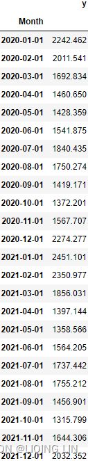

regressors = { 'Naive Forecaster' : NaiveForecaster( strategy='mean', 
                                                     sp=12
                                                   ),
               'Linear Regression': LinearRegression(),
               'K-NN Regressor': KNeighborsRegressor(n_neighbors=5),
               'Extra Tree Regressor': ExtraTreesRegressor(),
               'Random Forest Regressor': RandomForestRegressor(),
               'Gradient Boosting Regressor': GradientBoostingRegressor()
             }

for regName, reg in regressors.items():
    print( f'training {reg} ...' )
    
    predicted = make_forecast(train, len(test), regressor=reg , window=15)
    test[regName] = pd.Series( predicted.reshape(-1), 
                               index=test.index
                             )

for i in test.iloc[:, 1:]: # except y
    ax = df_en[-2*len(test):].plot(style='k--', alpha=0.45, title=i, figsize=(10,5))
    
    test[i].plot(ax=ax)
    plt.legend(['Actual', i])
    plt.show()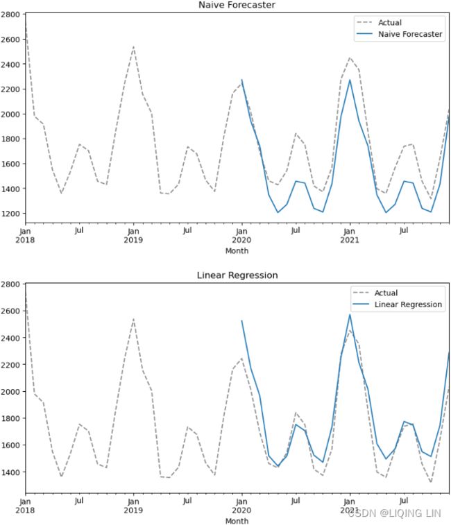

Visually, aside from the Naive Forecaster, all the models seem to perform well.

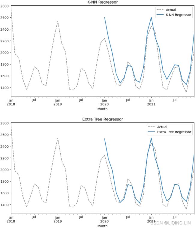
Figure 12.9 – Example of plotting each regressor's prediction against the actual data

Using performance metrics is a much better approach to evaluate the models numerically; for example, using MASE, sMAPE, MAPE, and RMSE, to name a few. Recall that Naive Forecaster is a baseline model from which we want to achieve better results.

Create the evaluate function that will evaluate all the models:

from sktime.performance_metrics.forecasting import( MeanSquaredError,
                                                    MeanAbsolutePercentageError,
                                                    MeanAbsoluteScaledError
                                                  )
mse = MeanSquaredError()
mape = MeanAbsolutePercentageError()
mase = MeanAbsoluteScaledError()

def evaluate( df, train, sort_by = 'MASE'):
    evals = pd.DataFrame( index=['sMAPE', 'MAPE', 'RMSE'] )
    y_truth = df['y']
    y_predicted = df.drop( columns=['y'] )
    for p in y_predicted:
        evals.loc['sMAPE', p] = mape( y_truth, y_predicted[p], symmetric=True )
        evals.loc['MAPE', p] = mape( y_truth, y_predicted[p], symmetric=False )
        evals.loc['RMSE', p] = np.sqrt( mse(y_truth, y_predicted[p]) )
        evals.loc['MASE', p] = mase( y_truth, y_predicted[p], y_train=train )
    return evals.T.sort_values(by=sort_by)

The function will return a sorted DataFrame by MASE (default) which can be updated to one of MAPE, RMSE, MASE, or sMAPE.

6. Call the function and pass the test and train sets:

evaluate(test, train)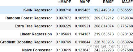

Figure 12.10 – Comparing the different regressor models

It looks like the KNN-Regressor model performed best, followed by the Random Forest model. Both models can handle non-linearity. Overall, all regressors did outperform the Naive Forecaster model.

Let's see how the ML models (regressors) compare against an ARIMA model using auto_arima from the pmdarima library. You explored auto_arima in the Forecasting time series data using auto_arima recipe from ts11_pmdarima_edgecolor_bokeh plotly_Prophet_Fourier_VAR_endog exog_Granger causality_IRF_Garch vola_LIQING LIN的博客-CSDN博客Chapter 11, Additional Statistical Modeling Techniques for Time Series.

You will use auto_arima to determine the best (p, d, q) orders for the non-seasonal components, and the (P, D, Q) orders for the seasonal components:

from pmdarima import auto_arima

n=len(test)
fh = ForecastingHorizon( np.arange(n)+1 ) # is_relative = None
arima = auto_arima( y=train, seasonal=True, m=12, # since it is a monthly dataset
                    suppress_warnings=True # test = 'kpss' (default)
                  ) #information_criterion='aic'(default) to select the best ARIMA model
arima.summary()

On the other hand, KPSS has the opposite null hypothesis, which assumes the time series is stationary.ts9_annot_arrow_hvplot PyViz interacti_bokeh_STL_seasonal_decomp_HodrickP_KPSS_F-stati_Box-Cox_Ljung_LIQING LIN的博客-CSDN博客

Once completed, you can examine the results with arima.summary() . The best model is SARIMAX(1, 1, 1) x (1, 0, 1, 12) =(p, d, q) x (P, D, Q, s).

# https://www.statsmodels.org/0.9.0/generated/statsmodels.tsa.statespace.mlemodel.MLEResults.test_serial_correlation.html#statsmodels.tsa.statespace.mlemodel.MLEResults.test_serial_correlation
# https://www.statsmodels.org/0.9.0/generated/statsmodels.tsa.statespace.mlemodel.MLEResults.html#statsmodels.tsa.statespace.mlemodel.MLEResults
results_sarima.test_serial_correlation('ljungbox', lags=1)

output – An array with (test_statistic, pvalue)

sigma squared represents the variance of the residual values(The error term is sigma2 or epsilon). This value is used to test the normality of residuals against the alternative of non-normality

where $\large \eta_t$ ∼WN(0, $\large \sigma^2$ ) is a white noise process
$\large \phi_q$ is coef term at time t-q: $\LARGE Y_t = c + \phi_1 e_{t-1} + \phi_2 e_{t-2} + ... \phi_q e_{t-q} + e_t$
SARIMAX(1, 1, 1) x (1, 0, 1, 12) =(p, d, q) x (P, D, Q, s).
Our lag variables are ma.L1, ar.S.L12 , ma.S.L12)
$\large (1-\phi_1B) (1-\Theta_1B^{12} ) (1-B)y_t = (1+\theta_1B) (1+\Theta_1B^{12})\varepsilon_t$ mpf6_Time Series Data_quandl_更正kernel PCA_AIC_BIC_trend_log_return_seasonal_decompose_sARIMAx_ADFull_LIQING LIN的博客-CSDN博客
ARIMA (p,d,q) : 8.5 Non-seasonal ARIMA models | Forecasting: Principles and Practice (2nd ed)

ARIMA(3,1,1) :
For example, an ARIMA(1,1, 1)(1,1, 1,4) model (without a constant) is for quarterly data (m=4), and can be written as $\large (1-\phi_1B) (1-\Theta_1B^4 ) (1-B)(1-B^4)y_t = (1+\theta_1B) (1+\Theta_1B^4)\varepsilon_t$

from statsmodels.tsa.statespace.sarimax import SARIMAX

model_sarima = SARIMAX( train, order=(0, 1, 1), seasonal_order=(1, 0, 1, 12) )
results_sarima = model_sarima.fit()
results_sarima.summary()

###############

We want to make sure each term in our model is statistically significant. The null for this section is that each coefficient is NOT statistically significant. Therefore, we want each term to have a p-value of less than 0.05, so we can reject the null hypothesis with statistically significant values.
In our example, Ll and L2 are not statistically significant as their p-values are above the 0.05 threshold.
###############

Ljung-Box

ts9_annot_arrow_hvplot PyViz interacti_bokeh_STL_seasonal_decomp_HodrickP_KPSS_F-stati_Box-Cox_Ljung_LIQING LIN的博客-CSDN博客

H0: The data are independently distributed (i.e. the correlations in the population from which the sample is taken are 0, so that any observed correlations in the data result from randomness of the sampling process).
Ha: The data are not independently distributed; they exhibit serial correlation.

$\large Q = T\sum_{k=1}^{h}r_k^2$ Box-Pierce test

h is the maximum lag being considered
- We suggest using h=10 for non-seasonal data and
- h=2m for seasonal data,
  - where m is the period of seasonality.
T is the number of observations or the sample size
is the (sample) autocorrelation at lag k.
- If each $\large r_k$ is close to zero, then Q will be small.
- If some $\large r_k$ values are large (positive or negative), then Q will be large.

However, the test is not good when h is large, so if these values are larger than T/5, then use h=T/5

$\large Q^{*} = T(T+2)\sum_{k=1}^{h}(T-k)^{-1}r^2_k$ (more accurate) Ljung-Box test

The null hypothesis $\large H_0$ for the Ljung-Box test states that the previous lags are not correlated with the current period. In other words, you are testing for the absence of autocorrelation.
large values of Q∗ suggest that the autocorrelations do not come from a white noise series(there is autocorrelation.).
Under $\large H_{0}$ the statistic Q asymptotically follows统计量 Q 渐近地遵循 a $\large \chi _{(h)}^{2}$ . For significance level α, the critical region for rejection of the hypothesis of randomness is: $\large Q > \chi^2_{1-\alpha,h}$
where $\large \chi _{1-\alpha ,h}^{2}$ is the (1 − α)-quantile[4] of the chi-squared distribution with h degrees of freedom.
The Ljung–Box test is commonly used in autoregressive integrated moving average (ARIMA) modeling. Note that it is applied to the residuals of a fitted ARIMA model, not the original series, and in such applications the hypothesis $\large H_0$ actually being tested is that the residuals from the ARIMA model have no autocorrelation. When testing the residuals of an estimated ARIMA model, the degrees of freedom need to be adjusted to reflect the parameter estimation. For example, for an ARIMA(p,0,q) model, the degrees of freedom should be set to h-p-q.
If the residuals are not independent, we can extract the non-randomness to make a better model.
Simulation studies have shown that the distribution for the Ljung–Box statistic is closer to a $\large \chi _{(h)}^{2}$ distribution than is the distribution for the Box–Pierce statistic for all sample sizes including small ones.

The Ljung Box test, pronounced “Young” and sometimes called the modified Box-Pierce test, tests that the errors are white noise.

# https://www.statsmodels.org/0.9.0/generated/statsmodels.tsa.statespace.mlemodel.MLEResults.test_serial_correlation.html#statsmodels.tsa.statespace.mlemodel.MLEResults.test_serial_correlation
# https://www.statsmodels.org/0.9.0/generated/statsmodels.tsa.statespace.mlemodel.MLEResults.html#statsmodels.tsa.statespace.mlemodel.MLEResults
results_sarima.test_serial_correlation('ljungbox', lags=1)

(test_statistic, pvalue)

The Ljung-Box (L1) (Q) is the LBQ test statistic at lag 1 is, the Prob(Q) is 9.08, and the p-value is 0. Since the p-value is lower than 0.05, we can reject the null hypothesis $\large H_0$ that the residuals from the ARIMA model have no autocorrelation.(reject that the previous lags are not correlated with the current period or the errors(residuals) are white noise; accept that the residuals from the ARIMA model are autocorrelated.)

If you’re interested in seeing all of the Ljung-Box test statistics and p-values for the lags, you can use a Ljung-Box diagnostic function.

from statsmodels.stats.diagnostic import acorr_ljungbox

acorr_ljungbox( results_sarima.resid, lags=12, return_df=True )

Heteroskedasticity异方差性

In statistics, the Breusch–Pagan test, developed in 1979 by Trevor Breusch and Adrian Pagan,[1] is used to test for heteroskedasticity in a linear regression model. it tests whether the variance of the errors from a regression is dependent on the values of the independent variables. In that case, heteroskedasticity is present.

Breusch and Pagan (1979) designed a test to confirm or reject the null assumption $\large H_0$ that the residuals from a regression are homogeneous, that is, with a constant volatility. The following formula represents their logic.
First, we run a linear regression of y against x:
$\large y_t = \beta_0 + \beta_1 x_t + \epsilon_t$ (6)

Here,

$\large y_t$ is the dependent variable,
$\large x_t$ is the independent variable,
$\large \beta_0$ is the intercept,
$\large \beta_1$ is the coefficient, and
$\large \epsilon_t$ is an error term.

and obtain from this fitted model a set of values for $\large \epsilon_t$ , the residuals. Ordinary least squares constrains these so that their mean is 0 and so,
given the assumption that their variance does not depend on the independent variables, an estimate of this variance can be obtained from the average of the squared values of the residuals $\large \epsilon_t ^ 2$ .
If the assumption is not held to be true, a simple model might be that the variance is linearly related to independent variables. Such a model can be examined by regressing the squared residuals on the independent variables对自变量的残差平方进行回归来检查, using an auxiliary regression equation of the form :

After we get the error term $\large \epsilon_t$ (residual or obtain a set of values of $\large \epsilon_t$ from this fitted model(6)), we run the second regression:
$\large \epsilon_t ^ 2 = \gamma_0 + \gamma_1 x_t + v_t$ (7)
This is the basis of the Breusch–Pagan test. It is a chi-squared test: the test statistic is distributed $\large n\chi^2$ with k degrees of freedom. If the test statistic has a p-value below an appropriate threshold (e.g. p < 0.05) then the null hypothesis $\large H_0$ of homoskedasticity is rejected and heteroskedasticity assumed.

If the Breusch–Pagan test shows that there is conditional heteroskedasticity, one could either use weighted least squares (if the source of heteroskedasticity is known) 使用加权最小二乘法（如果已知异方差的来源）or use heteroscedasticity-consistent standard errors或使用异方差一致的标准误差.

# https://www.statsmodels.org/0.9.0/generated/statsmodels.tsa.statespace.mlemodel.MLEResults.test_heteroskedasticity.html#statsmodels.tsa.statespace.mlemodel.MLEResults.test_heteroskedasticity
results_sarima.test_heteroskedasticity(method='breakvar',alternative='two-sided', use_f=True)

(test_statistic, pvalue)

Heteroscedasticity tests that the error residuals are homoscedastic or have the same variance. The summary performs White’s test. Our summary statistics show a test statistic of 1.77 and a p-value of 0.00, which means we reject the null hypothesis and our residuals show variance (standard deviation) is not constant.

Jarque-Bera

The test statistic JB is defined as $JB = \frac{n}{6} ( S^2 + \frac{1}{4}(K-3)^2 )$ and $\large S = \frac{\hat{u}_3}{\hat{\sigma}^3} = \frac{\frac{1}{n}\sum_{i=1}^{n}(x_i-\bar{x})^3}{(\frac{1}{n}\sum_{i=1}^{n}(x_i-\bar{x})^2)^{3/2}}$ and $\large K = \frac{\hat{u}_4}{\hat{\sigma}^4} = \frac{\frac{1}{n}\sum_{i=1}^{n}(x_i-\bar{x})^4}{(\frac{1}{n}\sum_{i=1}^{n}(x_i-\bar{x})^2)^{2}}$

where n is the number of data points, S is the sample skewness, and K is the sample kurtosis of the data.pff1_whylog return Nominal Inflation_CPI_Realized Volati_outlier_distplot_Jarque–Bera_pAcf_sARIMAx_LIQING LIN的博客-CSDN博客

Jarque-Bera tests for the normality of errors. It tests the null hypothesis $\large H_0$ that the data is normally distributed against an alternative of another distribution.

#https://www.statsmodels.org/0.9.0/generated/statsmodels.tsa.statespace.mlemodel.MLEResults.test_normality.html#statsmodels.tsa.statespace.mlemodel.MLEResults.test_normality
#https://www.statsmodels.org/0.9.0/generated/statsmodels.tsa.statespace.mlemodel.MLEResults.html#statsmodels.tsa.statespace.mlemodel.MLEResults
results_sarima.test_normality('jarquebera')

statsmodels.stats.stattools.jarque_bera — statsmodels 0.9.0 documentation

We see a test statistic of 70.21 $\large > \chi_{2,1-\alpha} =5.99$ (At 5% significant level(α = 0.05),) with a probability of 0 >0.05, which means we reject the null hypothesis, and the data is not normally distributed. Also, as part of the Jarque-Bera test, we see the distribution has a slight negative skew and a kurtosis.

How to Interpret ARIMA Results - Analyzing Alpha

Add the output predictions to the test DataFrame and run the evaluate function again:

n=len(test)
test['ARIMA'] = arima.predict(n)
test

evaluate(test,train)

This should produce a DataFrame with sorted models based on the MASE score:Figure 12.11 – Comparing the different ML models with ARIMA

You can plot the two best models to see how they compare visually:

train.loc['2011':].index

ax = train.loc['2011':].plot( style='--', alpha=0.35, figsize=(12,8) )
test['y'].plot(ax=ax, style='b--',)
test['ARIMA'].plot( ax=ax, style='k-.' )
test['K-NN Regressor'].plot( ax=ax, style='k-o' )
plt.legend(['train', 'test', 'ARIMA', 'K-NN Regressor'])
plt.show()

This should produce a time series plot showing the training data from January 2011 to August 2014, and the estimated forecasts from both the ARIMA model and the K-NN regression model from September 2014 to December 2021.

Figure 12.12 – Comparing K-NN regression with an ARIMA model

The ARIMA model did a decent尚好的,得体的 job overall compared to more advanced ML regressors. This is sometimes the case with smaller univariate time series. Keep in mind that the ML models (regressors) are not optimized yet (via hyperparameter tuning) while the ARIMA model was optimized by auto_arima to find the best hyperparameters (the seasonal and non-seasonal orders). ML algorithms are great for working with more complex multivariate time series data, as you will explore in the Forecasting with exogenous variables and ensemble learning recipe.

ML optimization with hyperparameter tuning is an essential step to ensure you are getting the best configuration and performance for the model of choice.

In this recipe, you used sklearn for running different regression models. What made this possible was using sktime's TransformedTargetForecaster class and the make_reduction function:

• To learn more about sktime's TransformedTargetForecaster for creating a pipeline, you can visit the documentation page here: TransformedTargetForecaster — sktime documentation.
• To learn more about the make_reduction function, you can visit the documentation page here: make_reduction — sktime documentation.

In the next recipe, you will explore how you can optimize an ML model.

Optimizing a forecasting model with hyperparameter tuning

ts12_Multi-step Forecast_sktime_bold_Linear Regress_sMAPE MASE_warn_plotly acf vlines_season_summary

Technical requirements

Understanding supervised machine learning

Preparing time series data for supervised learning

One-step forecasting using linear regression models with scikit-learn

MAPE(Mean Absolute Percentage Error)

SMAPE(Symmetric Mean Absolute Percentage Error)

MASE

Non seasonal time series

Seasonal time series

Non-time series data

plotly acf vlines

Regression Coefficients and Feature Selection

Multi-step forecasting using linear regression models with scikit-learn

Daily Temperature

Air Passengers

Energy Consumption

Forecasting using non-linear models with sktime

1. Basic forecasting workflows

Step 1 - Preparation of the data

ForecastingHorizon

Step 2 - Specifying the forecasting horizon

NaiveForecaster

Step 3 - Specifying the forecasting algorithm

Step 4 - Fitting the forecaster to the seen data

Step 5 - Requesting forecasts

1.2.2 Forecasters that require the horizon already in fit

1.2.3 Forecasters that can make use of exogeneous data

1.2.4. Multivariate forecasting

Deseasonalizer

PolynomialTrendForecaster

Detrender

make_reduction

TransformedTargetForecaster

Ljung-Box

Heteroskedasticity异方差性

Jarque-Bera

Optimizing a forecasting model with hyperparameter tuning

你可能感兴趣的:(人工智能,深度学习)

1.2.2 Forecasters that require the horizon already in `fit`