CIFAR-10数据集分类实验报告

本篇文章只是一篇CIFAR-10数据集分类简介，是我的一门课程的大作业，从BP网络进行分类到CNN进行分类。
程序贴在最后！！！

1 开发环境

目前主流的神经网络框架有Tensorflow，Pytorch，MXNET，Keras等。本次实验使用Pytroch深度学习框架。PyTorch看作加入了GPU支持的numpy，并且它是一个拥有自动求导功能的强大的深度神经网络。

2 BP神经网络相关知识

2.1 激活函数

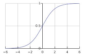
• 激活函数的作用是加入非线性因素,从而提高神经网络对模型的表达能力,解决线性模型所不能解决的问题。
  
  

• 上图是sigmoid激活函数。

• 计算量大，反向传播求误差梯度时，求导涉及除法。

• 反向传播时，很容易就会出现梯度消失的情况，从而无法完成深层网络的训练。
  
  

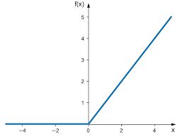
• 上图是ReLU激活函数。

• ReLU 的收敛速度会比 sigmoid 快很多。

2.2 损失函数

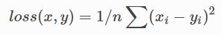
• MSE损失更适合用于回归问题，比如房价预测，对于分类问题，MSE Loss不能很好的逼近目标。
  
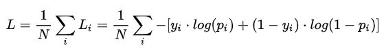
• 交叉熵损失，以二分类为例。该损失更适合用于分类问题。

3 CIFAR-10数据集

• 该数据集分为训练集和测试集，一共有10种动物。其中，训练集有50000张图片，测试集有10000张图片，训练集和测试集不重叠，图片大小为32 * 32 * 3。

4 BP网络实验

• SGD（随机梯度下降）优化策略。SGD就是每一次随机抽取一个mini-batch，迭代计算mini-batch的梯度，然后对参数进行更新。weight decay（权重衰减）：设置为5e-4,防止过拟合，是放在正则项（regularization）前面的一个系数，正则项一般指示模型的复杂度。momentum（动量）：设置为0.9，提高收敛速度。学习率设置为0.01，ReLU实验的学习率为0.005。
• 引入Batchsize，设置为128，通过并行化提高内存的利用率。就是尽量让你的GPU满载运行，提高训练速度；适当Batch Size使得梯度下降方向更加准确。
• 输入是将32 * 32 * 3的图像展平为3072维的图像特征，输出是10维。
• 总共学习100个epochs。
• 从隐藏层神经元个数、激活函数和隐藏层层数三个角度实验，证明对BP网络的影响。
• 实验并没有对学习率有一个很好的调整，只是大范围的确定了学习率，所以训练的精度不代表模型最好精度。

4.1 三层BP网络隐藏层神经元个数

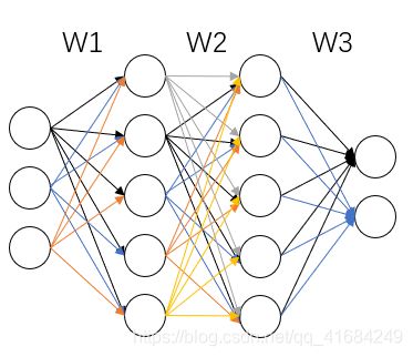
• 如图，是三层BP网络，使用sigmoid激活函数，将损失函数改为交叉熵损失，而不是使用均方差MSE损失。
  

• 上图是确定三层BP网络确定隐藏层神经元个数的经验。
  
  

• 如图，对三层BP网络的隐藏层分别设置为8，2048和10240个神经元。

• 对于隐藏层设置为8个神经元，神经元个数太少会导致网络表达能力太弱，无法对特征进行正确的表达。

• 对于隐藏层设置为10240个神经元，神经元个数太多不一定就能够对特征有正确的表达，而且神经元个数过大容易导致模型泛化能力较差。

• 由上述经验确定的隐藏层设置为2048个神经元，效果最好。
  
  

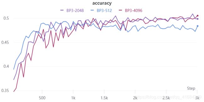
• 分别选择512，2048，4096个神经元，可以看到512个神经元相对于2048和4096个神经元稍微差一点，而2048和4096个神经元效果相似。

4.2 激活函数Sigmoid和ReLU

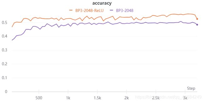
• 使用三层BP网络实验，隐藏层神经元个数为2048，该实验只改变了两个模型的激活函数。
• 可以看到ReLU激活函数明显优于Sigmoid激活函数。
• ReLU收敛速度更快，且能使损失收敛到一个更小的值。
  
  
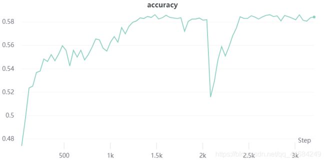
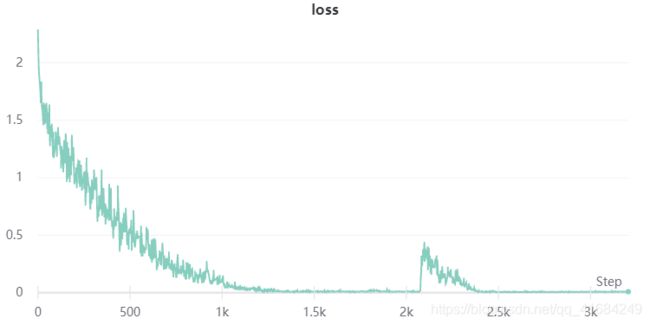
• 注意这里有一个尖峰，损失突然增大，我个人的理解是我只固定了一个学习率，当损失很小的适合应该使用小学习率。

4.3 隐藏层层数

• 四层BP网络，隐藏层增加一层。隐藏层的神经元个数为2048。
  
  

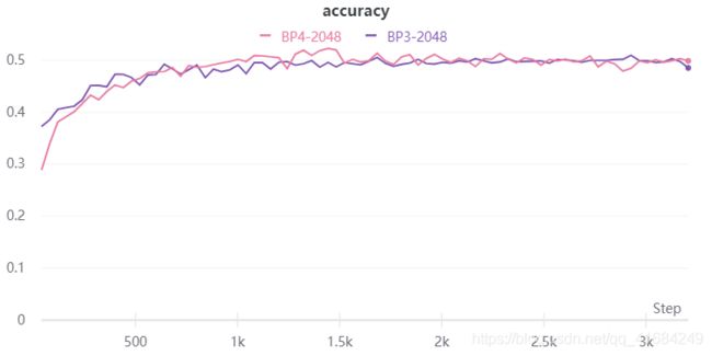
• 如图所示，粉色和紫色分别表示4层BP网络和3层BP网络，他们使用Sigmoid激活函数。

• 层数的增加反而训练收敛速度变慢，看测试准确率几乎相似，，说明层数增加并没有对特征有个更好的非线性表示，这有可能是我参数没调好，也有可能是Sigmoid激活函数两端梯度为0，梯度不均匀，训练不稳定。
  
  

• 在上述实验基础上，将Sigmoid函数改为ReLU函数，可以看到，层数增加，模型的收敛速度更快，精度更高，能更好的表示非线性。

5 卷积神经网络

• BP网络实验我将图片的像素展平为32 * 32 * 3的数组，将该数组作为这张图片的特征。实际上可以将分类问题实际上是特征提取之后加全连接层进行分类，这里提取特征就可以使用效率更高的CNN卷积神经网络。
  

5.1 LeNet-5

• 首先进行卷积操作，提取图片特征后，将特征展平用全连接层进行分类。
  
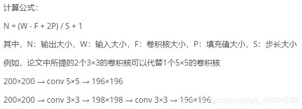
• 网络结构，假设原来图像大小32 * 32 * 3，conv1将其变为16 * 16 * 6，conv2经过第一个Conv卷积核变为12 * 12 * 16，然后经过MaxPool变为6 * 6 * 16，然后输入到全连接层。

5.2 自制CNN

    def __init__(self):
        super(CNN, self).__init__()
        self.conv1 = nn.Sequential(
            nn.Conv2d(3, 8, 3, 1, 1),
            nn.ReLU(),
            nn.MaxPool2d(2)
        )
        self.conv2 = nn.Sequential(
            nn.Conv2d(8, 16, 3, 1, 1),
            nn.ReLU(),
            nn.MaxPool2d(2)
        )
        self.conv3 = nn.Sequential(
            nn.Conv2d(16, 32, 3, 1, 1),
            nn.ReLU(),
            nn.MaxPool2d(2)
        )
        self.conv4 = nn.Sequential(
            nn.Conv2d(32, 64, 3, 1, 1),
            nn.ReLU(),
            nn.MaxPool2d(2)
        )
        self.fc1 = nn.Sequential(
            nn.Linear(64 * 2 * 2, 120),
            nn.ReLU()
        )
        self.fc2 = nn.Sequential(
            nn.Linear(120, 84),
            nn.ReLU()
        )
        self.fc3 = nn.Linear(84, 10)

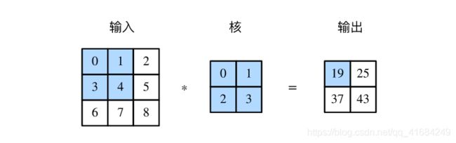
• 使用大小为3的卷积核

5.3 实验

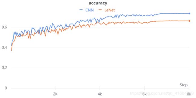
• 如图，使用卷积神经网络效果要远远好于BP网络。

6 代码

import torch
from torch.utils import data
import torch.nn as nn
from tqdm import tqdm
import wandb
import torchvision.transforms as transforms
import torchvision

class BP_model(nn.Module):
    def __init__(self):
        super(BP_model, self).__init__()
        self.fc1 = nn.Linear(32 * 32 * 3, 2048) # 线性层
        self.fc2 = nn.Linear(2048, 2048)
        self.fc3 = nn.Linear(2048, 10)

    def forward(self, x):
        out = x.view(-1, 32 * 32 * 3) # 展平处理
        out = nn.ReLU()(self.fc1(out))
        out = nn.ReLU()(self.fc2(out))
        out = self.fc3(out)
        return out

class LeNet5(nn.Module):
    def __init__(self):
        super(LeNet5, self).__init__()
        self.conv1 = nn.Sequential(
            nn.Conv2d(3, 6, 5, 1, 2), # 卷积核 原来通道数 转换后通道数 卷积核大小 步长 填充
            nn.ReLU(), # 激活函数
            nn.MaxPool2d(2) # 最大池化层
        )
        self.conv2 = nn.Sequential(
            nn.Conv2d(6, 16, 5, 1, 0),
            nn.ReLU(),
            nn.MaxPool2d(2)
        )
        self.fc1 = nn.Sequential(
            nn.Linear(16 * 6 * 6, 120),
            nn.ReLU()
        )
        self.fc2 = nn.Sequential(
            nn.Linear(120, 84),
            nn.ReLU()
        )
        self.fc3 = nn.Linear(84, 10)
    def forward(self, x):
        x = self.conv1(x)
        x = self.conv2(x)
        x = x.view(-1, 16 * 6 * 6)
        x = self.fc1(x)
        x = self.fc2(x)
        x = self.fc3(x)
        return x

class CNN(nn.Module):
    def __init__(self):
        super(CNN, self).__init__()
        self.conv1 = nn.Sequential(
            nn.Conv2d(3, 8, 3, 1, 1),
            nn.ReLU(),
            nn.MaxPool2d(2)
        )
        self.conv2 = nn.Sequential(
            nn.Conv2d(8, 16, 3, 1, 1),
            nn.ReLU(),
            nn.MaxPool2d(2)
        )
        self.conv3 = nn.Sequential(
            nn.Conv2d(16, 32, 3, 1, 1),
            nn.ReLU(),
            nn.MaxPool2d(2)
        )
        self.conv4 = nn.Sequential(
            nn.Conv2d(32, 64, 3, 1, 1),
            nn.ReLU(),
            nn.MaxPool2d(2)
        )
        self.fc1 = nn.Sequential(
            nn.Linear(64 * 2 * 2, 120),
            nn.ReLU()
        )
        self.fc2 = nn.Sequential(
            nn.Linear(120, 84),
            nn.ReLU()
        )
        self.fc3 = nn.Linear(84, 10)
    def forward(self, x):
        x = self.conv1(x)
        x = self.conv2(x)
        x = self.conv3(x)
        x = self.conv4(x)
        x = x.view(-1, 64 * 2 * 2)
        x = self.fc1(x)
        x = self.fc2(x)
        x = self.fc3(x)
        return x

if __name__ == '__main__':

    wandb.init(project="BP")
    wandb.config.dropout = 0.2
    wandb.config.hidden_layer_size = 128
    # 读取数据，数据预处理
    transform = transforms.Compose([
                transforms.ToTensor(),
                transforms.Normalize((0.4914, 0.4822, 0.4465), (0.2023, 0.1994, 0.2010))]) # totensor是将0-255转到0-1，normalize是将0-1转换到-1-1
    trainset = torchvision.datasets.CIFAR10(root='./data', train=True,
                                            download=False, transform=transform) # 读取数据集，数据预处理
    trainloader = torch.utils.data.DataLoader(trainset, batch_size=128,
                                              shuffle=True, num_workers=1, pin_memory=True) # 打乱，包装成batchsize
    testset = torchvision.datasets.CIFAR10(root='./data', train=False,
                                           download=False, transform=transform)
    testloader = torch.utils.data.DataLoader(testset, batch_size=128,
                                             shuffle=False, num_workers=1, pin_memory=True)

    device = torch.device("cuda:0") # 选择cpu或者GPU
    # model = BP_model()
    # model = LeNet5() # 用哪个模型，打开哪个，屏蔽另外两个
    model = CNN()
    model.to(device) # 选择cpu或者gpu
    criterion = nn.CrossEntropyLoss() # 交叉熵损失
    optimizer = torch.optim.SGD([{'params': model.parameters()}],
                                lr=0.005, weight_decay=5e-4, momentum=0.9) # 随机梯度优化策略
    scheduler = torch.optim.lr_scheduler.CosineAnnealingLR(optimizer, T_max=200) # CNN训练使用该学习率优化策略，bp网络也可以使用试试

    for epoch in range(80):
        # 训练
        model.train()
        for i, (img, label) in tqdm(enumerate(trainloader)):
            img, label = img.to(device, non_blocking=True), label.to(device, non_blocking=True).long() # 加载数据
            output = model(img) # 计算结果
            loss = criterion(output, label) # 计算损失
            optimizer.zero_grad()
            loss.backward() # 反向传播
            optimizer.step() # 优化器更新

            iters = epoch * len(trainloader) + i
            if iters % 10 == 0:
                wandb.log({'loss': loss}) # 可视化
        # 测试
        accuracy = 0
        model.eval()
        for i, (img, label) in enumerate(testloader):
            img, label = img.to(device), label.to(device).long()
            output = model(img)
            output = output.max(dim=1)[1] # 预测是哪一类
            accuracy += (output==label).sum().item() # 准确率计算
        accuracy = accuracy / 10000 # 准确率计算
        print(accuracy)
        wandb.log({'accuracy': accuracy}) # 可视化

        scheduler.step() # 学习率更新