【Tensoflow2】Unet实现CityScapes语义分割及resize插值问题
文章目录
- 1.数据介绍
- 2.Unet模型
- 3.开发流程
-
- 1).读取数据及数据预处理
- 2).函数式模型构建
- 3).模型编译及训练
- 4).Resize插值问题
1.数据介绍
- 本文主要使用Tensorflow2实现Unet模型在城市景观数据场景下的语义分割实现。使用数据为CityScapes,数据主页:https://www.cityscapes-dataset.com/。数据分为原图,分割图,并包含训练集及测试集。

- 语义分割后数据输出共34类。每一类为单独的物体,不同物体标注不同的颜色。
| 物体名称 | 输出类型ID | 颜色 |
|---|---|---|
| unlabeled | 0 | ( 0, 0, 0) |
| ego vehicle | 1 | ( 0, 0, 0) |
| rectification border | 2 | ( 0, 0, 0) |
| out of roi | 3 | ( 0, 0, 0) |
| static | 4 | ( 0, 0, 0) |
| dynamic | 5 | (111, 74, 0) |
| ground | 6 | ( 81, 0, 81) |
| road | 7 | (128, 64,128) |
| sidewalk | 8 | (244, 35,232) |
| parking | 9 | (250,170,160) |
| rail track | 10 | (230,150,140) |
| building | 11 | ( 70, 70, 70) |
| wall | 12 | (102,102,156) |
| fence | 13 | (190,153,153) |
| guard rail | 14 | (180,165,180) |
| bridge | 15 | (150,100,100) |
| tunnel | 16 | (150,120, 90) |
| pole | 17 | (153,153,153) |
| polegroup | 18 | (153,153,153) |
| traffic light | 19 | (250,170, 30) |
| traffic sign | 20 | (220,220, 0) |
| vegetation | 21 | (107,142, 35) |
| terrain | 22 | (152,251,152) |
| sky | 23 | ( 70,130,180) |
| person | 24 | (220, 20, 60) |
| rider | 25 | (255, 0, 0) |
| car | 26 | ( 0, 0,142) |
| truck | 27 | ( 0, 0, 70) |
| bus | 28 | ( 0, 60,100) |
| caravan | 29 | ( 0, 0, 90) |
| trailer | 30 | ( 0, 0,110) |
| train | 31 | ( 0, 80,100) |
| motorcycle | 32 | ( 0, 0,230) |
| bicycle | 33 | (119, 11, 32) |
2.Unet模型
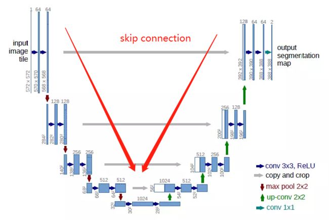
- Unet模型是广泛用于无人驾驶,医学影像语义分割场景的基础模型。Unet使用编码器-解码器的U型结构,左半部分下采样进行特征工程,右半部分上采样结合skip connection融合特征。最后输出每个像素的分类(此处共34类)。
3.开发流程
1).读取数据及数据预处理
- 导包
import tensorflow as tf
from tensorflow import keras
from tensorflow.keras import layers
import numpy as np
import glob
import matplotlib.pyplot as plt
- 加载数据,乱序
注意:如果使用Kaggle NoteBook进行训练,图片及语义分割图像不一一对应
# 训练集
train_path_raw = glob.glob(r'D:\tensorflowDataSet\cityUNET\image2\images\train\*\*.png')
train_label_path_raw = glob.glob(r'D:\tensorflowDataSet\cityUNET\gtFine\train\*\*gtFine_labelIds.png')
# 测试集
test_path_raw = glob.glob(r'D:\tensorflowDataSet\cityUNET\image2\images\val\*\*.png')
test_label_path_raw = glob.glob(r'D:\tensorflowDataSet\cityUNET\gtFine\val\*\*gtFine_labelIds.png')

train_total_num = len(train_path_raw) #2975
test_total_num = len(test_path_raw)   #500
# 打乱数据集
index = np.random.permutation(train_total_num)
train_path = np.array(train_path)[index]
train_label_path = np.array(train_label_path)[index]
- 图片预处理,原始图片像素为(2048,1024),考虑到显存,统一resize到(256,256),并使用图像增强。
def read_image(path): # 加载原始图像
    image = tf.io.read_file(path)
    image = tf.image.decode_png(image,channels=3)
    return image

def read_label(path): # 加载语义分割图像
    image = tf.io.read_file(path)
    image = tf.image.decode_png(image,channels=1)
    return image

def crop_img(image,mask):      # 图像增强,随机剪裁为(256,256)

    img = tf.concat([image,mask],axis=-1)#将原图和语义图合并剪裁
    # resize成(256,256),插值方法用邻近插值(为啥要用临近插值?后续会讲)
    img = tf.image.resize(img,(280, 280),method=tf.image.ResizeMethod.NEAREST_NEIGHBOR)
    img = tf.image.random_crop(img,size=[256,256,4])

    return img[:,:,:3],img[:,:,3:]

def normalize(image,mask):    #归一化到[-1,1],加速训练
    image = tf.cast(image,tf.float32) /127.5 - 1
    mask = tf.cast(mask,tf.int32)
    return image,mask

def image_handler_train(image_path,label_path): #训练集加载
    train_img = read_image(image_path)
    label_img = read_label(label_path)

    image,mask = crop_img(train_img,label_img)

    if tf.random.uniform(()) > 0.5: #图像增强-随机左右翻转
        image = tf.image.flip_left_right(image)
        mask = tf.image.flip_left_right(mask)

    if tf.random.uniform(()) > 0.5: #图像增强-明暗度
        image = tf.image.adjust_brightness(image,0.5)
        mask = tf.image.adjust_brightness(mask,0.5)

    image,mask = normalize(image,mask)
    return image,mask

def image_handler_test(image_path,label_path):  #测试集加载(不需要进行增强)
    train_img = read_image(image_path)
    label_img = read_label(label_path)

    train_img = tf.image.resize(train_img,size=(256,256),method=tf.image.ResizeMethod.NEAREST_NEIGHBOR)
    label_img = tf.image.resize(label_img,size=(256,256),method=tf.image.ResizeMethod.NEAREST_NEIGHBOR)

    image,mask = normalize(train_img,label_img)
    return image,mask
- 构建数据集
BUFFERSIZE = 100
BATCHSIZE = 20
AUTO = tf.data.experimental.AUTOTUNE #自动加载
#构建训练集
train_path_dataset = tf.data.Dataset.from_tensor_slices((train_path,train_label_path))
train_dataset = train_path_dataset.map(image_handler_train,num_parallel_calls=AUTO)
train_dataset = train_dataset.repeat().shuffle(BUFFERSIZE).batch(BATCHSIZE).prefetch(AUTO)
#构建测试集
test_path_dataset = tf.data.Dataset.from_tensor_slices((test_path,test_label_path))
test_dataset = test_path_dataset.map(image_handler_test,num_parallel_calls=AUTO)
test_dataset = test_dataset.batch(BATCHSIZE)
2).函数式模型构建
- 模型构建的时候可以根据Unet一层一层的写,也可以使用模型组合的方式。
# 按照Unet模型一层一层写
def make_unet_model():
    input = keras.Input(shape=(256,256,3))
    x1 = layers.Conv2D(64,3,strides=1,padding='same')(input)
    x1 = layers.BatchNormalization()(x1)
    x1 = layers.ReLU()(x1)
    x1 = layers.Conv2D(64,3,strides=1,padding='same')(x1)
    x1 = layers.BatchNormalization()(x1)
    x1 = layers.ReLU()(x1)  #(256,256,64)

    x2 = layers.MaxPooling2D()(x1) #(128,128,64)

    x2 = layers.Conv2D(128,3,strides=1,padding='same')(x2)
    x2 = layers.BatchNormalization()(x2)
    x2 = layers.ReLU()(x2)
    x2 = layers.Conv2D(128,3,strides=1,padding='same')(x2)
    x2 = layers.BatchNormalization()(x2)
    x2 = layers.ReLU()(x2)  #(128,128,128)

    x3 = layers.MaxPooling2D()(x2) #(64,64,128)

    x3 = layers.Conv2D(256,3,strides=1,padding='same')(x3)
    x3 = layers.BatchNormalization()(x3)
    x3 = layers.ReLU()(x3)
    x3 = layers.Conv2D(256,3,strides=1,padding='same')(x3)
    x3 = layers.BatchNormalization()(x3)
    x3 = layers.ReLU()(x3) #(64,64,256)

    x4 = layers.MaxPooling2D()(x3) #(32,32,256)

    x4 = layers.Conv2D(512,3,padding='same',strides=1)(x4)
    x4 = layers.BatchNormalization()(x4)
    x4 = layers.ReLU()(x4)
    x4 = layers.Conv2D(512,3,padding='same',strides=1)(x4)
    x4 = layers.BatchNormalization()(x4)
    x4 = layers.ReLU()(x4) #(32,32,512)

    x5 = layers.MaxPooling2D()(x4) #(16,16,512)

    x5 = layers.Conv2D(1024,3,padding='same',strides=1)(x5)
    x5 = layers.BatchNormalization()(x5)
    x5 = layers.ReLU()(x5)
    x5 = layers.Conv2D(1024,3,padding='same',strides=1)(x5)
    x5 = layers.BatchNormalization()(x5)
    x5 = layers.ReLU()(x5) #(16,16,1024)

    x4_ = layers.Conv2DTranspose(512,2,padding='same',strides=2)(x5)
    x4_ = layers.BatchNormalization()(x4_)
    x4_ = layers.ReLU()(x4_) #(32,32,512)

    x3_ = tf.concat([x4,x4_],axis=-1) #(32,32,1024)
    x3_ = layers.Conv2D(512,3,padding='same',strides=1)(x3_)
    x3_ = layers.BatchNormalization()(x3_)
    x3_ = layers.ReLU()(x3_)
    x3_ = layers.Conv2D(512,3,padding='same',strides=1)(x3_)
    x3_ = layers.BatchNormalization()(x3_)
    x3_ = layers.ReLU()(x3_) #(32,32,512)

    x3_= layers.Conv2DTranspose(256,2,padding='same',strides=2)(x3_)
    x3_ = layers.BatchNormalization()(x3_)
    x3_ = layers.ReLU()(x3_) #(64,64,256)

    x2_ = tf.concat([x3,x3_],axis=-1) #(64,64,512)
    x2_ = layers.Conv2D(256,3,padding='same',strides=1)(x2_)
    x2_ = layers.BatchNormalization()(x2_)
    x2_ = layers.ReLU()(x2_)
    x2_ = layers.Conv2D(256,3,padding='same',strides=1)(x2_)
    x2_ = layers.BatchNormalization()(x2_)
    x2_ = layers.ReLU()(x2_) #(64,64,256)

    x2_ = layers.Conv2DTranspose(128,2,padding='same',strides=2)(x2_)
    x2_ = layers.BatchNormalization()(x2_)
    x2_ = layers.ReLU()(x2_) #(128,128,128)

    x1_ = tf.concat([x2,x2_],axis=-1) #(128,128,256)
    x1_ = layers.Conv2D(128,3,padding='same',strides=1)(x1_)
    x1_ = layers.BatchNormalization()(x1_)
    x1_ = layers.ReLU()(x1_)
    x1_ = layers.Conv2D(128,3,padding='same',strides=1)(x1_)
    x1_ = layers.BatchNormalization()(x1_)
    x1_ = layers.ReLU()(x1_) #(128,128,128)

    x1_= layers.Conv2DTranspose(64,2,padding='same',strides=2)(x1_)
    x1_ = layers.BatchNormalization()(x1_)
    x1_ = layers.ReLU()(x1_) #(256,256,64)

    x_ = tf.concat([x1,x1_],axis=-1) #(256,256,128)
    x_ = layers.Conv2D(64,3,padding='same',strides=1)(x_)
    x_ = layers.BatchNormalization()(x_)
    x_ = layers.ReLU()(x_)
    x_ = layers.Conv2D(64,3,padding='same',strides=1)(x_)
    x_ = layers.BatchNormalization()(x_)
    x_ = layers.ReLU()(x_) #(256,256,64)
	#输出层,共34类
    output = layers.Conv2D(34,1,padding='same',strides=1,activation='softmax')(x_) #(256,256,34)

    return keras.Model(inputs=input,outputs=output)
- 使用模型组合构建模型
# 构建基础模型
def down_sample(filters,kernel):  #下采样卷积层
   model = keras.Sequential()
   model.add(layers.Conv2D(filters,kernel,strides=1,padding='same'))
   model.add(layers.BatchNormalization())
   model.add(layers.ReLU())
   return model

def max_pooling():                #下采样池化层
   model = keras.Sequential()
   model.add(layers.MaxPooling2D())
   return model

def up_sample(filters,kernel):    #上采样卷积层
   model = keras.Sequential()
   model.add(layers.Conv2DTranspose(filters,kernel,padding='same',strides=2))
   model.add(layers.BatchNormalization())
   model.add(layers.ReLU())
   return model
def get_unet_model():
    input = keras.Input(shape=(256,256,3)) #(256,256,3)

    down_models = [
        down_sample(64,3), #(256,256,64)
        down_sample(64,3),
        max_pooling(),     #(128,128,64)
        down_sample(128,3),#(128,128,128)
        down_sample(128,3),
        max_pooling(),     #(64,64,128)
        down_sample(256,3),#(64,64,256)
        down_sample(256,3),
        max_pooling(),     #(32,32,256)
        down_sample(512,3),#(32,32,512)
        down_sample(512,3),
        max_pooling(),     #(16,16,512)
        down_sample(1024,3),#(16,16,1024)
        down_sample(1024,3)#(16,16,1024)
    ]

    down_output = []
    x = input
    for i,down in enumerate(down_models):
        x = down(x)
        if i % 3 == 1:
            down_output.append(x)

    down_output = reversed(down_output[:-1])

    up_models = [
        up_sample(512,2),
        up_sample(256,2),
        up_sample(128,2),
        up_sample(64,2)
    ]

    up_conv2_model_1 = [
        down_sample(512,3),
        down_sample(256,3),
        down_sample(128,3),
        down_sample(64,3)
    ]

    up_conv2_model_2 = [
        down_sample(512,3),
        down_sample(256,3),
        down_sample(128,3),
        down_sample(64,3)
    ]

    for d_out,up,conv2_1,conv2_2 in zip(down_output,up_models,up_conv2_model_1,up_conv2_model_2):
        x = up(x)
        x = tf.concat([d_out,x],axis=-1)
        x = conv2_1(x)
        x = conv2_2(x)
    #输出层,共34类
    x = layers.Conv2D(34,1,padding='same',strides=1,activation='softmax')(x)

    return keras.Model(inputs=input,outputs=x)
#构建模型
model = get_unet_model()
3).模型编译及训练
- 模型评估指标
i) acc:分类正确率。
ii) MeanIou:交集与并集之比,越大拟合效果越好。
#重写__call__方法,MeanIou默认按照OneHot进行计算。
class MeanIoU(tf.keras.metrics.MeanIoU):
   def __call__(self, y_true, y_pred, sample_weight=None):
       y_pred = tf.argmax(y_pred, axis=-1)
       return super().__call__(y_true, y_pred, sample_weight=sample_weight)
- 模型编译
model.compile(optimizer='adam',
               loss='sparse_categorical_crossentropy',
               metrics=['acc',MeanIoU(num_classes=34)])
- 模型训练
EPOCHS = 80
train_step = train_total_num // BATCHSIZE
val_step = test_total_num // BATCHSIZE

history = model.fit(train_dataset,
           epochs=EPOCHS,
           steps_per_epoch= train_step,
           validation_data=test_dataset,
           validation_steps=val_step)
-
指标可视化
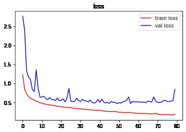
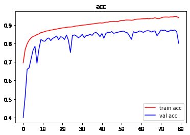
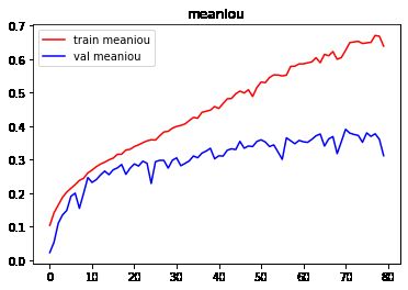
-
结论
由图像可以看出,训练严重过拟合,建议使用Dropout抑制过拟合。测试集表现不佳,建议增加训练数据集,使用图像增强。 -
模型预测
第一列为原始图像,第二列为标签分割图,第三列为预测图像。

4).Resize插值问题
- 在对图像进行resize时,使用了tf.image.ResizeMethod.NEAREST_NEIGHBOR邻近插值法,其实不仅有这种插值法,如图:
class ResizeMethod(object):
 BILINEAR = 'bilinear' #双线性
 NEAREST_NEIGHBOR = 'nearest' #最近邻插值法
 BICUBIC = 'bicubic'  #双三次插值
 AREA = 'area' #区域插值
 LANCZOS3 = 'lanczos3' #领域采样插值
 LANCZOS5 = 'lanczos5'
 GAUSSIAN = 'gaussian'
 MITCHELLCUBIC = 'mitchellcubic'
- 这里为啥要选择邻近插值法,邻近插值法在resize之后不会改变在标签数据的像素类型(目标数据34类)。
label_img = read_image(test_label_path_raw[1])

label_img = tf.image.resize(label_img,size=(256,256),method=tf.image.ResizeMethod.NEAREST_NEIGHBOR)
np.unique(label_img.numpy())
# output[ 1,  2,  3,  4,  7,  8,  9, 11, 13, 17, 20, 21, 23, 25, 26, 33]


#以下插值法可能会影响分类。
label_img = tf.image.resize(label_img,size=(256,256),method=tf.image.ResizeMethod.BILINEAR)
np.unique(label_img.numpy())
# output[ 1.  ,  1.25,  1.5 ,  1.75,  2.  ,  2.5 ,  3.  ,  3.25,  4.  ,4.5 ,  5.5 ,  6.5 ,  6.75,  7.  ,  7.25,  7.5 ,  7.75,  8. ......]


label_img = tf.image.resize(label_img,size=(256,256),method=tf.image.ResizeMethod.AREA)
np.unique(label_img.numpy())
# output[ 1.  ,  1.03125,  1.0625 ,  1.09375,  1.125  ,  1.15625, 1.1875 ,  1.21875,  1.25   ,  1.28125,  1.34375,  1.375  ...]
- Opencv图像插值法算法及比较