《TensorFlow深度学习》（五）——神经网络

本文是书籍《TensorFlow深度学习》的学习笔记之一

神经网络

本节我们通过替换感知机的激活函数，同时并行堆叠多个神经元来实现多输入、多输出的如下网络层结构。

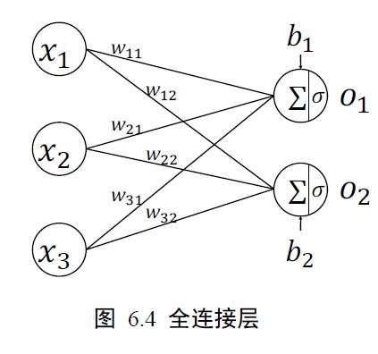
第一个输出节点的输出为：
1 = (11 ∙ 1 + 21 ∙ 2 + 1 ∙ + 1)
第二个输出节点的输出为：
2 = (12 ∙ 1 + 22 ∙ 2 + 2 ∙ + 2)

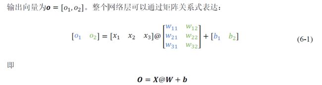
考虑并行计算，即有多个样本，则增加一行输入x，增加一行输出o：

下面有两种实现方式，一种是张量：

x = tf.random.normal([2,784])# 两个样本，每个长度为784
w1 = tf.Variable(tf.random.truncated_normal([784,256],stddev=0.1))
b1 = tf.Variable(tf.zeros([256))
o1 = tf.matmul(x,w1)+b1
o1 = tf.nn.relu(o1)

一种是层：

x = tf.random.normal([4,28*28])
from tensorflow.keras import layers # 导入层模块
# 创建全连接层，指定输出节点数和激活函数
fc = layers.Dense(512, activation=tf.nn.relu)
h1 = fc(x) # 通过fc 类实例完成一次全连接层的计算，返回输出张量

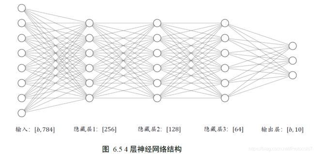
以上是实现单层神经网络的方法，要实现如下的多层神经网络，也有两种方法。

张量：

# 隐藏层1 张量
w1 = tf.Variable(tf.random.truncated_normal([784, 256], stddev=0.1))
b1 = tf.Variable(tf.zeros([256]))
# 隐藏层2 张量
w2 = tf.Variable(tf.random.truncated_normal([256, 128], stddev=0.1))
b2 = tf.Variable(tf.zeros([128]))
# 隐藏层3 张量
w3 = tf.Variable(tf.random.truncated_normal([128, 64], stddev=0.1))
b3 = tf.Variable(tf.zeros([64]))
# 输出层张量
w4 = tf.Variable(tf.random.truncated_normal([64, 10], stddev=0.1))
b4 = tf.Variable(tf.zeros([10]))

with tf.GradientTape() as tape: # 梯度记录器
	# x: [b, 28*28]
	# 隐藏层1 前向计算，[b, 28*28] => [b, 256]
	h1 = x@w1 + tf.broadcast_to(b1, [x.shape[0], 256])
	h1 = tf.nn.relu(h1)
	# 隐藏层2 前向计算，[b, 256] => [b, 128]
	h2 = h1@w2 + b2
	h2 = tf.nn.relu(h2)
	# 隐藏层3 前向计算，[b, 128] => [b, 64]
	h3 = h2@w3 + b3
	h3 = tf.nn.relu(h3)
	# 输出层前向计算，[b, 64] => [b, 10]
	h4 = h3@w4 + b4

层：

# 导入常用网络层layers
from tensorflow.keras import layers,Sequential
fc1 = layers.Dense(256, activation=tf.nn.relu) # 隐藏层1
fc2 = layers.Dense(128, activation=tf.nn.relu) # 隐藏层2
fc3 = layers.Dense(64, activation=tf.nn.relu) # 隐藏层3
fc4 = layers.Dense(10, activation=None) # 输出层

x = tf.random.normal([4,28*28])
h1 = fc1(x) # 通过隐藏层1 得到输出
h2 = fc2(h1) # 通过隐藏层2 得到输出
h3 = fc3(h2) # 通过隐藏层3 得到输出
h4 = fc4(h3) # 通过输出层得到网络输出

对于这种数据依次向前传播的网络，也可以通过Sequential 容器封装成一个网络大类对象，调用大类的前向计算函数一次即可完成所有层的前向计算，使用起来更加方便，实现如下：

# 导入Sequential 容器
from tensorflow.keras import layers,Sequential
# 通过Sequential 容器封装为一个网络类
model = Sequential([
layers.Dense(256, activation=tf.nn.relu) , # 创建隐藏层1
layers.Dense(128, activation=tf.nn.relu) , # 创建隐藏层2
layers.Dense(64, activation=tf.nn.relu) , # 创建隐藏层3
layers.Dense(10, activation=None) , # 创建输出层
])

前向计算时只需要调用一次网络大类对象，即可完成所有层的按序计算：out = model(x) # 前向计算得到输出

接下来我们设计输出层：
❑ ∈ ^ 输出属于整个实数空间，或者某段普通的实数空间，比如函数值趋势的预测，年龄的预测问题等。
❑ ∈ [0,1] 输出值特别地落在[0, 1]的区间，如图片生成，图片像素值一般用[0, 1]区间的值表示；或者二分类问题的概率，如硬币正反面的概率预测问题。
❑ ∈ [0, 1], ∑ = 1 输出值落在[0,1]的区间，并且所有输出值之和为 1，常见的如多分类问题，如MNIST 手写数字图片识别，图片属于10 个类别的概率之和应为1。
❑ ∈ [−1, 1] 输出值在[-1, 1]之间

不同情况的解决方案书中有，略。

最后我们进行误差计算。

1. 均方差(Mean Squared Error，简称MSE)误差函数把输出向量和真实向量映射到笛卡尔坐标系的两个点上，通过计算这两个点之间的欧式距离(准确地说是欧式距离的平方)来衡量两个向量之间的差距：

o = tf.random.normal([2,10]) # 构造网络输出
y_onehot = tf.constant([1,3]) # 构造真实值
y_onehot = tf.one_hot(y_onehot, depth=10)
loss = keras.losses.MSE(y_onehot, o) # 计算均方差

特别要注意的是，MSE 函数返回的是每个样本的均方差，需要在样本维度上再次平均来获得平均样本的均方差，实现如下：loss = tf.reduce_mean(loss) # 计算batch 均方差

实战

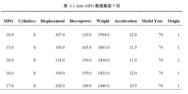
本节我们将利用全连接网络模型来完成汽车的效能指标MPG(Mile Per Gallon，每加仑燃油英里数)的预测问题实战。

# %%
from __future__ import absolute_import, division, print_function, unicode_literals

import pathlib
import os

os.environ['TF_CPP_MIN_LOG_LEVEL'] = '2'

import matplotlib.pyplot as plt
import pandas as pd
import seaborn as sns

import tensorflow as tf

from tensorflow import keras
from tensorflow.keras import layers, losses

print(tf.__version__)

# 在线下载汽车效能数据集
dataset_path = keras.utils.get_file("auto-mpg.data",
                                    "http://archive.ics.uci.edu/ml/machine-learning-databases/auto-mpg/auto-mpg.data")

# 效能（公里数每加仑），气缸数，排量，马力，重量
# 加速度，型号年份，产地
column_names = ['MPG', 'Cylinders', 'Displacement', 'Horsepower', 'Weight',
                'Acceleration', 'Model Year', 'Origin']
raw_dataset = pd.read_csv(dataset_path, names=column_names,
                          na_values="?", comment='\t',
                          sep=" ", skipinitialspace=True)

dataset = raw_dataset.copy()
# 查看部分数据
dataset.tail()
dataset.head()
dataset
# %%


# %%

# 统计空白数据,并清除
dataset.isna().sum()
dataset = dataset.dropna()
dataset.isna().sum()
dataset
# %%

# 处理类别型数据，其中origin列代表了类别1,2,3,分布代表产地：美国、欧洲、日本
# 其弹出这一列
origin = dataset.pop('Origin')
# 根据origin列来写入新列
dataset['USA'] = (origin == 1) * 1.0
dataset['Europe'] = (origin == 2) * 1.0
dataset['Japan'] = (origin == 3) * 1.0
dataset.tail()

# 切分为训练集和测试集
train_dataset = dataset.sample(frac=0.8, random_state=0)
test_dataset = dataset.drop(train_dataset.index)

# %% 统计数据
sns.pairplot(train_dataset[["Cylinders", "Displacement", "Weight", "MPG"]],
             diag_kind="kde")
# %%
# 查看训练集的输入X的统计数据
train_stats = train_dataset.describe()
train_stats.pop("MPG")
train_stats = train_stats.transpose()
train_stats

# 移动MPG油耗效能这一列为真实标签Y
train_labels = train_dataset.pop('MPG')
test_labels = test_dataset.pop('MPG')


# 标准化数据
def norm(x):
    return (x - train_stats['mean']) / train_stats['std']


normed_train_data = norm(train_dataset)
normed_test_data = norm(test_dataset)
# %%

print(normed_train_data.shape, train_labels.shape)
print(normed_test_data.shape, test_labels.shape)


# %%

class Network(keras.Model):
    # 回归网络
    def __init__(self):
        super(Network, self).__init__()
        # 创建3个全连接层
        self.fc1 = layers.Dense(64, activation='relu')
        self.fc2 = layers.Dense(64, activation='relu')
        self.fc3 = layers.Dense(1)

    def call(self, inputs, training=None, mask=None):
        # 依次通过3个全连接层
        x = self.fc1(inputs)
        x = self.fc2(x)
        x = self.fc3(x)

        return x


model = Network()
model.build(input_shape=(None, 9))
model.summary()
optimizer = tf.keras.optimizers.RMSprop(0.001)
train_db = tf.data.Dataset.from_tensor_slices((normed_train_data.values, train_labels.values))
train_db = train_db.shuffle(100).batch(32)

# # 未训练时测试
# example_batch = normed_train_data[:10]
# example_result = model.predict(example_batch)
# example_result


train_mae_losses = []
test_mae_losses = []
for epoch in range(200):
    for step, (x, y) in enumerate(train_db):

        with tf.GradientTape() as tape:
            out = model(x)
            loss = tf.reduce_mean(losses.MSE(y, out))
            mae_loss = tf.reduce_mean(losses.MAE(y, out))

        if step % 10 == 0:
            print(epoch, step, float(loss))

        grads = tape.gradient(loss, model.trainable_variables)
        optimizer.apply_gradients(zip(grads, model.trainable_variables))

    train_mae_losses.append(float(mae_loss))
    out = model(tf.constant(normed_test_data.values))
    test_mae_losses.append(tf.reduce_mean(losses.MAE(test_labels, out)))

plt.figure()
plt.xlabel('Epoch')
plt.ylabel('MAE')
plt.plot(train_mae_losses, label='Train')

plt.plot(test_mae_losses, label='Test')
plt.legend()

# plt.ylim([0,10])
plt.legend()
plt.savefig('auto.svg')
plt.show()

# %%

实验结果：
对于回归问题，我们还可以用MAE（Mean Absolute Error，平均绝对误差）来测试性能。