使用MLP进行负荷预测

一、简单介绍

      Multi-layer Perceptron（MLP），即多层感知器，是一个前馈式的、具有监督的人工神经网络结构。通过多层感知器可包含多个隐藏层，实现对非线性数据的分类建模。MLP将数据分为训练集、测试集、检验集。其中，训练集用来拟合网络的参数，测试集防止训练过度，检验集用来评估网络的效果，并应用于总样本集。当因变量是分类型的数值，MLP神经网络则根据所输入的数据，将记录划分为最适合类型。常被MLP用来进行学习的反向传播算法，在模式识别的领域中算是标准监督学习算法，并在计算神经学及并行分布式处理领域中，持续成为被研究的课题。MLP已被证明是一种通用的函数近似方法，可以被用来拟合复杂的函数，或解决分类问题。

二、源代码分享

      首先查看气象数据各字段的缺失情况，从数据中了解到，天气类型、风向、风速、降雨量四个字段数据缺失严重，这里使用各字段的中位数替换异常数据，经过检查，符合数据仅有局部零星几个缺失数据，由于负荷数据在相邻的几天内，固定时间段的波动较小，这里处理缺失值的方法是：使用前一个非缺失值来填充缺失值。

import torch
import numpy as np
import pandas as pd
import matplotlib.pyplot as plt
import warnings; warnings.simplefilter('ignore')
torch.__version__
path = '../data/STLF_DATA_IN_1.xls'
df_load = pd.read_excel(path,sheet_name=0,header=None)
df_weather = pd.read_excel(path, sheet_name=1, header=None)
plt.figure()
# plt.rcParams['font.sans-serif']=['SimHei']
weather_type = df_weather[1].value_counts(sort=True)
weather_type.plot.bar()
plt.savefig('../img/weather_type.png')
df_weather = df_weather.drop(df_weather[df_weather[1] == "天气类型"].index)
df_weather = df_weather.drop(df_weather[df_weather[1] == "风向"].index)
df_weather = df_weather.drop(df_weather[df_weather[1] == "风速"].index)
df_weather = df_weather.drop(df_weather[df_weather[1] == "降雨量"].index)
weather_type = df_weather[1].value_counts(sort=True)
weather_type.plot.bar()
plt.savefig('../img/weather_type2.png')
df_max_tempe = df_weather.loc[df_weather[1] == "最高温度", [0, 2]]
df_min_tempe = df_weather.loc[df_weather[1] == "最低温度", [0, 2]]
df_avg_tempe = df_weather.loc[df_weather[1] == "平均温度", [0, 2]]
df_humidity = df_weather.loc[df_weather[1] == "湿度", [0, 2]]

df_weather2 = pd.merge(df_max_tempe, df_min_tempe, how='left', on=[0, 0])
df_weather2 = pd.merge(df_weather2, df_avg_tempe, how='left', on=[0, 0])
df_weather2 = pd.merge(df_weather2, df_humidity, how='left', on=[0, 0])

df_weather2.isna().sum()
df_weather2.describe()
df_weather2.columns = [0, 'max_tempe', 'min_tempe', 'avg_tempe', 'humidity']
df_weather2.boxplot(column=['avg_tempe'])
df_weather2['min_tempe'][df_weather2['min_tempe'] < -800] = df_weather2['min_tempe'].median()
df_weather2['avg_tempe'][df_weather2['avg_tempe'] < -40] = df_weather2['avg_tempe'].median()
df_weather2['humidity'][df_weather2['humidity'] < -8000] = df_weather2['humidity'].median()
df_weather2['humidity'][df_weather2['humidity'] > 2000] = df_weather2['humidity'].median()

df_load = df_load.drop(df_load.tail(1).index)
df_load.describe()
column_list = list(range(1, 97))
plt.figure(figsize=(18,6))
df_load.boxplot(column=column_list,figsize=(20, 4))
plt.savefig('../img/load_boxplot.png')
for i in range(1, 5):
    df_load[i][df_load[i] == 0] = df_load[i].median()
    print(df_load.isna().sum())
df_load = df_load.fillna(axis=0, method='ffill')
df_data = pd.merge(df_load, df_weather2, how='left', on=[0, 0])
for column in ['max_tempe', 'min_tempe', 'avg_tempe', 'humidity']:
    index = df_data[column][df_data[column].isna()].index
    for idx in index:
        if idx - 365 > 0:
            df_data.at[idx, column] = df_data.at[idx - 365, column]
        else:
            df_data.at[idx, column] = df_data.at[idx + 2 * 365, column]
    # print(index)
    df_data.isna().sum()
    from pandas.tseries.holiday import USFederalHolidayCalendar as calendar
from chinese_calendar import is_holiday
cal = calendar()
holidays = cal.holidays(start=df_data[0].min(), end=df_data[0].max())
def my_isholiday(s):
    if s < pd.Timestamp('2004-01-01'):
        return s in holidays
    else:
        return is_holiday(s)
        
df_data[0] = pd.to_datetime(df_data[0], format='%Y%m%d')
df_data['type_of_day'] = df_data[0].apply(lambda s : s.dayofweek).astype('object')
df_data['holiday'] = df_data[0].apply(my_isholiday).astype('object')
df_data = pd.get_dummies(df_data)

data_norm = df_data.iloc[:, 1:].values.astype('float64', copy=False)
data_norm[:, :96] = (data_norm[:, :96] / 7000)
data_norm[:, 96:99] = data_norm[:, 96:99] / 20
data_norm[:, 99] = data_norm[:, 99] / 100
print(data_norm.shape)
Y = data_norm[7:, :96]
X = np.zeros((1975, 685))
for idx in range(7, len(data_norm)):
    X[idx-7] = np.append(data_norm[idx-7:idx, :96], data_norm[idx, 96:])
np.savetxt('../data/features.csv', X, delimiter=",")
np.savetxt('../data/labels.csv', Y, delimiter=",")
labels = torch.tensor(Y, dtype=torch.float32)
labels = labels.to('cuda')
features = torch.tensor(X, dtype=torch.float32)
features = features.to('cuda')
import torch.nn as nn
from torch.nn import init

def get_net(num_inputs=685, num_hiddens1 = 520, num_outputs=96):
    net = nn.Sequential(
        nn.Linear(num_inputs, num_hiddens1),
        nn.ReLU(),
        nn.Linear(num_hiddens1, num_outputs)
    )
    for params in net.parameters():
        init.normal_(params, mean=0, std=0.01)
    net.to('cuda')
    return net
def accuary(y_pred, y_real):
    return 1 - np.sqrt(np.mean(((y_pred - y_real) / y_real) ** 2, axis=1))
def train(net, train_features, train_labels, test_features, test_labels, 
          num_epochs, learning_rate, batch_size):
    train_ls, test_ls = [], []
    train_accus, test_accus = [], []
    best_test_accu = 0
    dataset = torch.utils.data.TensorDataset(train_features, train_labels)
    train_iter = torch.utils.data.DataLoader(dataset, batch_size, shuffle=True)
    optimizer = torch.optim.Adam(params=net.parameters(), lr=learning_rate) 
    net = net.float()
    for epoch in range(num_epochs):
        net.train(True)
        for X, y in train_iter:
            loss = torch.nn.MSELoss()
            l = loss(net(X.float()), y.float())
            optimizer.zero_grad()
            l.backward()
            optimizer.step()
        train_ls.append(l)
        net.eval()
        train_accu = accuary(net(train_features).detach().cpu().numpy(), train_labels.detach().cpu().numpy())
        train_accus.append(train_accu.mean())
        if test_labels is not None:
            test_l = loss(net(test_features), test_labels)
            test_ls.append(test_l)
            test_accu = accuary(net(test_features).detach().cpu().numpy(), test_labels.detach().cpu().numpy())
            test_accus.append(test_accu.mean())
            if test_accu.mean() > best_test_accu:
                torch.save(net, './model.pt')
                best_test_accu = test_accu.mean()
        if epoch % 10 == 0:
            print('epooch %d: train mse %.4f, test mes %.4f, train accuary %.4f, test accuary %.4f' % (epoch, l, test_l, train_accu.mean(), test_accu.mean()))
    return train_ls, test_ls, train_accus, test_accus
train_index = np.arange(0, len(X)-155)
test_index = np.arange(len(X)-155, len(X))
train_feautures = features[train_index]
train_labels = labels[train_index]
test_feautures = features[test_index]
test_labels = labels[test_index]
net = get_net()
print(net)
num_epochs, learning_rate, batch_size = 1000, 1e-3, 32
train_ls, test_ls, train_accus, test_accus= train(net, train_feautures, train_labels, test_feautures, test_labels, num_epochs, learning_rate, batch_size)
plt.figure(figsize=(10, 8), dpi=100)
plt.plot(train_ls, label='train')
plt.plot(test_ls, label='test')
plt.legend()
plt.xlabel('epoch')
plt.ylabel('mse')
plt.title('Train and test mse curve')
plt.savefig('../img/train_test_mse.png')

plt.figure(figsize=(10, 8), dpi=100)
plt.plot(train_accus, label='train')
plt.plot(test_accus, label='test')
plt.xlabel('epoch')
plt.ylabel('accuary')
plt.title('Train and test accuary curve')
plt.legend()
plt.savefig('../img/train_test_accu.png')
best_epoch = np.array(test_ls).argmin()
print('test best mse: %.6f' % test_ls[best_epoch])
print('test best accuary: ', test_accus[best_epoch])

      负荷预测

from torch import load, Tensor
import pandas as pd
import numpy as np
from chinese_calendar import is_holiday
import matplotlib.pyplot as plt
import warnings

warnings.simplefilter('ignore')

print('Loading data...')
df_load = pd.read_excel('../data/STLF_DATA_IN_1.xls', sheet_name=0, header=None)
df_weather = pd.read_excel('../data/STLF_DATA_IN_1.xls', sheet_name=1, header=None)


predict_date = int(input('请输入待预测日（示例：20080605）：'))
date = pd.to_datetime(predict_date, format='%Y%m%d')
load_index = df_load.loc[df_load[0] == predict_date].index.item()
load_data = df_load.iloc[load_index-7:load_index, 1:].values.reshape((1, -1)) / 7000


max_tempe = df_weather.loc[(df_weather[0] == predict_date) & (df_weather[1] == '最高温度'), [2]].values / 20
min_tempe = df_weather.loc[(df_weather[0] == predict_date) & (df_weather[1] == '最低温度'), [2]].values / 20
avg_tempe = df_weather.loc[(df_weather[0] == predict_date) & (df_weather[1] == '平均温度'), [2]].values / 20
humidity = df_weather.loc[(df_weather[0] == predict_date) & (df_weather[1] == '湿度'), [2]].values / 100
weather_data = np.concatenate([max_tempe, min_tempe, avg_tempe, humidity]).reshape((1, -1))


type_of_day = np.eye(7)[date.dayofweek]
holiday = np.eye(2)[int(is_holiday(date))]
time_data = np.concatenate([type_of_day, holiday]).reshape((1, -1))


features = np.concatenate([load_data, weather_data, time_data], axis=1).reshape(1, 685)
features = Tensor(features)

print('Loading model...')
net = load('./model.pt', map_location='cpu')

print('Start predicting...')
net.eval()
labels = net(features).detach().numpy() * 7000

print('Start ploting...')
plt.figure(figsize=(10, 8))
plt.title(predict_date)
plt.xlabel('Time')
plt.ylabel('Load/MW')
plt.plot(labels.reshape(96))
plt.grid()

print('Done!')

三、结果讲解

      数据集中总共有1982条数据，这里选择2008.1.1-2008.6.4的数据作为验证集（即后155条数据），经过不断的训练&验证，最终的超参数选择如下：

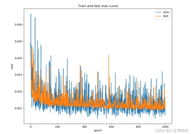
      训练集和验证集的mse曲线
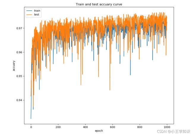
      训练集和验证集的精度曲线

      在第942次迭代中，获得了最优模型，模型效果如下：

      验证集精度最高的一天：

      验证集预测精度箱线图与散点图


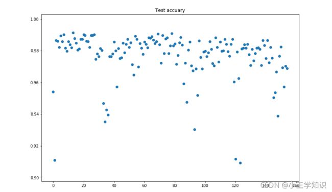
      通过分析可知，模型对节假日以及其他负荷水平突然变化的情况，预测精度不够高。根据上面的低精度天数据的分析，提出改进想法，对节假日单独建模，单独预测使用其他更适合于时间序列分析的模型比如LSTM、GRU等

      本次实验搭建了一个MLP模型，其输入为前七天的负荷数据与待预测日的气象、时间特征数据，输出为待预测日的负荷数据。经过训练，模型在验证集共155条数据的平均预测精度为97.66%，其中有10条数据预测精度低于95%，原因主要是节假日负荷水平突变。