目标检测之GFL

前言

论文地址：https://arxiv.org/pdf/2006.04388.pdf
本博客的讲解代码：https://github.com/open-mmlab/mmdetection
源码：https://github.com/implus/GFocal

1.GFL的主要创新部分

Generalized Focal Loss: Learning Qualified and Distributed Bounding Boxes for Dense Object Detection
论文通过分析预测输出时的分类，回归和定位质量评估的表示，发现他们之间存在一些问题：

• classification score 和 IoU/centerness score 训练测试不一致（如FCOS的分类分数和中心预测分数）。
  bbox regression 采用的表示不够灵活，没有办法建模复杂场景下的uncertainty
  为了解决这两个问题，作者给这三种预测输出表示设计了新的representations，并提出了Generalized Focal Loss来优化网络。

提出了两种新的表征方式：
将分类分数和检测框质量分数结合，得到分类-质量联合分数，标签变为连续值。
bbox边框的回归值由单一确定值（狄拉克分布）变为一定范围的任意概率分布。
提出了两种新的Focal Loss损失函数：

Quality Focal Loss 对分类-质量联合分数连续值标签进行优化。
Distribution Focal Loss 对边界框的任意概率分布进行优化。
具体可以看原作者的解析：https://zhuanlan.zhihu.com/p/147691786
或者：https://zhuanlan.zhihu.com/p/310229973

2.结合代码体现创新部分

1.训练阶段的预测输出

这部分分数预测输出不变，主要是回归框的变化

    def forward_single(self, x, scale):
        """Forward feature of a single scale level.

        Args:
            x (Tensor): Features of a single scale level.
            scale (:obj: `mmcv.cnn.Scale`): Learnable scale module to resize
                the bbox prediction.

        Returns:
            tuple:
                cls_score (Tensor): Cls and quality joint scores for a single
                    scale level the channel number is num_classes.
                bbox_pred (Tensor): Box distribution logits for a single scale
                    level, the channel number is 4*(n+1), n is max value of
                    integral set.
        """
        cls_feat = x
        reg_feat = x
        for cls_conv in self.cls_convs:
            cls_feat = cls_conv(cls_feat)
        for reg_conv in self.reg_convs:
            reg_feat = reg_conv(reg_feat)
        cls_score = self.gfl_cls(cls_feat)
        bbox_pred = scale(self.gfl_reg(reg_feat)).float()	# 注意这里输出C的变化[B,4*(16+1),H,W]
        return cls_score, bbox_pred

这里，gfl的head部分，self.gfl_reg()输出的是一个一定数量的离散框的回归值。一定数量：表示的是每条边的预测回归输出为(self.reg_max + 1)倍，作者实验得出self.reg_max =16为最佳。

self.gfl_reg = nn.Conv2d(self.feat_channels, 4 * (self.reg_max + 1), 3, padding=1)	# (256,4*(16+1),3)

2.将bbox边框的回归值由单一确定值（狄拉克分布）变为一定范围的任意概率分布。

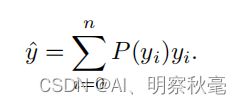
作者使用softmax函数实现离散形式的任意分布。$P_i$表示用softmax函数使预测值变为0-1的概率，$y_i$从所给的边框范围（16）均匀取值，这样就从一个回归问题变为一个“多分类问题”。

通过self.integral(pos_bbox_pred)来变化分布

pos_bbox_pred_corners = self.integral(pos_bbox_pred)    # [N,4]

这里注释解释的很清楚，就是通过一个任意分布+一个线性变换来确定预测的回归框lrtb值

class Integral(nn.Module):
    """A fixed layer for calculating integral result from distribution.

    This layer calculates the target location by :math: `sum{P(y_i) * y_i}`,
    P(y_i) denotes the softmax vector that represents the discrete distribution
    y_i denotes the discrete set, usually {0, 1, 2, ..., reg_max}

    Args:
        reg_max (int): The maximal value of the discrete set. Default: 16. You
            may want to reset it according to your new dataset or related
            settings.
    """

    def __init__(self, reg_max=16):
        super(Integral, self).__init__()
        self.reg_max = reg_max
        self.register_buffer('project',
                             torch.linspace(0, self.reg_max, self.reg_max + 1))  #

    def forward(self, x):
        """Forward feature from the regression head to get integral result of
        bounding box location.

        Args:
            x (Tensor): Features of the regression head, shape (N, 4*(n+1)),
                n is self.reg_max.

        Returns:
            x (Tensor): Integral result of box locations, i.e., distance
                offsets from the box center in four directions, shape (N, 4).
        """
        x = F.softmax(x.reshape(-1, self.reg_max + 1), dim=1)
        x = F.linear(x, self.project.type_as(x)).reshape(-1, 4)
        return x

每条边的任意分布为{$x_i:p_i$},$x_i$表示预测的离散lrtb的值，$p_i$表示它们离散值对应的分布概率。输入x经过F.softmax处理后就是对应的$p_i$。
self.project：给了一个0-16的17个间距为1的值。用来表示边框周围的范围。

F.linear(x, self.project.type_as(x)).reshape(-1, 4)

将每条边的17个预测值通过概率分布预测出一个值，最后重新变为常见的4个lrtb预测输出。

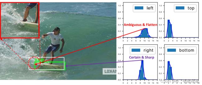
从这个图可以看出，一些检测对象的边界并非十分明确。对于滑板左侧被水花模糊，引起对左边界的预测分布是任意而扁平的，对右边界的预测分布是明确而尖锐的。

3.Distribution Focal Loss

    需要获得的分布虽然不再像狄拉克分布那么极端，但也应该在标签值附近。因此作者提出Distribution Focal Loss损失函数，目的让网络快速聚焦到标签附近的数值，使标签处的概率密度尽量大。思想是使用交叉熵函数，来优化标签y附近左右两个位置的概率，使网络分布聚焦到标签值附近。

def distribution_focal_loss(pred, label):
"""
    Args:
        pred (torch.Tensor): Predicted general distribution of bounding boxes
            (before softmax) with shape (N, n+1), n is the max value of the
            integral set `{0, ..., n}` in paper.
        label (torch.Tensor): Target distance label for bounding boxes with
            shape (N,).

    Returns:
        torch.Tensor: Loss tensor with shape (N,).
    """
    dis_left = label.long()     # 转换为长整型，向下取整。偏向左边的值，label:是ltrb格式
    dis_right = dis_left + 1	# 偏向右边的值
    weight_left = dis_right.float() - label   # 小数，公式里的（y_{i+1}-y）
    weight_right = label - dis_left.float()		# （y-y_{i}）
    #F.cross_entropy会对输入的pred进行softmax，dis_left为pre进行log_softmax后的索引
    loss = F.cross_entropy(pred, dis_left, reduction='none') * weight_left \
        + F.cross_entropy(pred, dis_right, reduction='none') * weight_right
    return loss

4.Quality Focal Loss

由下图可知，就是联合分类和IOU：预测的box与target box的IOU值作为监督的label，这样label值由一个0，1的离散值，变为0-1的连续值.所以计算分类Loss的时候，是通过分类和IOU的联系进行优化。

score[pos_inds] = bbox_overlaps(    # 没传中心置信度，是将预测的box与target box的IOU值作为置信度分数
                pos_decode_bbox_pred.detach(),
                pos_decode_bbox_targets,
                is_aligned=True)

计算分类分数的时候将score传入，好进行分类-质量联合分数Loss的计算
# cls (qfl) loss
loss_cls = self.loss_cls(
    cls_score, (labels, score),
    weight=label_weights,
    avg_factor=num_total_samples)

公式中，原始的Fcoal loss针对的标签是离散值（y=0或y=1），这里提出的分类-检测框质量联合表示，其标签y为[0,1]的连续值，σ为预测值。

def quality_focal_loss(pred, target, beta=2.0):
"""
    Args:
        pred (torch.Tensor): Predicted joint representation of classification
            and quality (IoU) estimation with shape (N, C), C is the number of
            classes.
        target (tuple([torch.Tensor])): Target category label with shape (N,)
            and target quality label with shape (N,).
        beta (float): The beta parameter for calculating the modulating factor.
            Defaults to 2.0.

    Returns:
        torch.Tensor: Loss tensor with shape (N,).
    """
    assert len(target) == 2, """target for QFL must be a tuple of two elements,
        including category label and quality label, respectively"""
    # label denotes the category id, score denotes the quality score
    label, score = target
	# 负样本的loss为什么要单独出来计算呢？这里没太明白
    # negatives are supervised by 0 quality score,负样本用0去监督
    pred_sigmoid = pred.sigmoid()   # 前面都没用过sigmod
    scale_factor = pred_sigmoid     # [N,c]
    zerolabel = scale_factor.new_zeros(pred.shape)  #[N,c]
    loss = F.binary_cross_entropy_with_logits(	# 自带sigmod的交叉熵，传入后会对pred进行sigmod
        pred, zerolabel, reduction='none') * scale_factor.pow(beta)  #这里其实全部样本都用0监督了，后面正样本部分会被替换掉

    # FG cat_id: [0, num_classes -1], BG cat_id: num_classes
    bg_class_ind = pred.size(1)
    pos = ((label >= 0) & (label < bg_class_ind)).nonzero().squeeze(1)	#正样本
    pos_label = label[pos].long()	#[pos,]
    # positives are supervised by bbox quality (IoU) score，正样本的
    scale_factor = score[pos] - pred_sigmoid[pos, pos_label]
    loss[pos, pos_label] = F.binary_cross_entropy_with_logits(
        pred[pos, pos_label], score[pos],
        reduction='none') * scale_factor.abs().pow(beta)

    loss = loss.sum(dim=1, keepdim=False)
    return loss

5.后处理部分

        for cls_score, bbox_pred, stride, anchors in zip(
                cls_scores, bbox_preds, self.anchor_generator.strides,
                mlvl_anchors):
            assert cls_score.size()[-2:] == bbox_pred.size()[-2:]
            assert stride[0] == stride[1]
            scores = cls_score.permute(0, 2, 3, 1).reshape(
                batch_size, -1, self.cls_out_channels).sigmoid()   # sigmoid,[N,HWC]
            bbox_pred = bbox_pred.permute(0, 2, 3, 1)   # [N,H,W,4*(16+1)]
            bbox_pred = self.integral(bbox_pred) * stride[0]   # [N,H,W,4]
            bbox_pred = bbox_pred.reshape(batch_size, -1, 4)    # [N,HW4]

bbox_pred = self.integral(bbox_pred) * stride[0] # [N,H,W,4]不同之处只需使用self.integral变换回原来的lrtb格式就行。

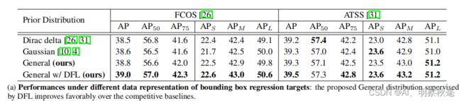
3.消融实验

1.QFL

2.DFL

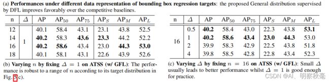
这里对DFL中取合适的数量和间隔进行了实验。

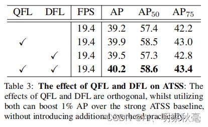
3.QFL+DFL

总结

十分优秀论文和研究工作！作者在论文后面还有些数据分析，值得阅读。并且作者后续已经发布了GFLV2,基于V1的情况下，利用学习到的bbox的分布来指导分类-质量评估的生成，能带来几乎无损涨点。后续有时间应该会介绍下GFLV2。
博客里所说都是个人理解，欢迎大家进行留言讨论！