Mask R-CNN算法详解（二）

Mask R-CNN详解+个人理解（附代码）（二）

在上一章中我们讲到，Mask R-CNN是基于Faster R-CNN的优化版本，而其中最主要的优化在于，它在Faster R-CNN的基础上：加了一个Mask Prediction Branch (Mask 预测分支)，并且改良了ROI Pooling，提出了ROI Align。我们先看看两种神经网络的结构图来进行对比：

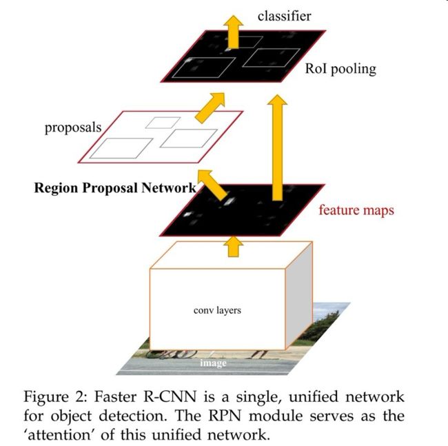
图一 Faster R-CNN结构图

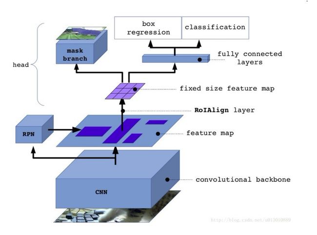
图二 Mask R-CNN结构图

二、Mask R-CNN的部件解读

（一）、convolutional backbone

（二）、FPN（Feature Pyramid Network）

先贴出关于FPN的经典论文，提供给有兴趣的读者参考：
https://arxiv.org/abs/1612.03144 （Feature Pyramid Networks for Object Detection）
FPN，即Feature Pyramid NetWork，特征金字塔网络，最初提出是为了改进CNN的特征提取，以及feature maps的融合，该论文在Fast/Faster R-CNN上进行实验，在Mask R-CNN中也延用了。金字塔结构的优势是其产生的特征每一层都是语义信息加强的，包括高分辨率的低层。

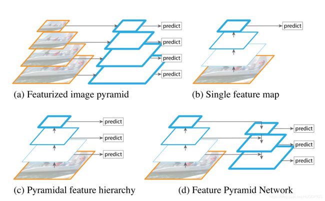
图三 几种不同的金字塔特征提取结构

首先看看这张图片，这张图片讲述了从图片金字塔网络到特征金字塔网络的各种金字塔网络形式：
（a）：图a是最原始的图像金字塔网络，原理是将图像做成不同尺寸，然后将不同尺寸的图像生成对应不同尺寸的特征，显然，时间成本大大增加了。这种方法所使用的特征通常是传统图像处理领域的特征，而面对深度网络的训练时，图像金字塔常常使GPU力不从心。
（b）：图b体现的是单个特征图，同时是网络最后一层的特征。我们知道不同层的特征图尺度就不同，金字塔的特征提取结构虽不错，但是前后层之间由于不同深度影响，语义信息差距太大，主要是高分辨率的低层特征很难有代表性的检测能力，所以在某些模型结构中，我们仅使用最后一层的特征。例如：SPP Net，Fast R-CNN，Faster R-CNN。
（c）：图c的来源是我们熟知的SSD，它更像是一种介于图a与图b之间的折中选择，它参考a，b的原理后保留了特征金字塔中高层的特征，高分辨率低层，同时，没有使用上采样减少了计算资源的多余使用，但是他丢弃了分辨率最高的低层特征，导致在小目标的检测效果不理想。
（d）：图d是我们主要阐述的特征金字塔网络，也就是在Mask R-CNN中所使用的金字塔结构，顶层特征通过上采样和低层特征做融合，而且每层都是独立预测的。

FPN的提出是为了实现更好的feature maps融合，当仅使用最后一层的feature maps时，虽然最后一层的feature maps 语义强，但是位置和分辨率都比较低，容易检测不到比较小的物体。FPN的功能就是融合了底层到高层的feature maps ，从而充分的利用了提取到的各个阶段的特征（ResNet中的C2-C5）。

这张图片充分地体现了FPN的运行模式，把更抽象，语义更强的高层特征图进行上取样，然后把该特征横向连接（lateral connections ）至前一层特征，因此高层特征得到加强（图中的2x up）。而在我们融合特征图的时候，横向连接的两层特征要保证相同的空间尺寸（图中的1x1 conv）。

把高层特征做2倍上采样（最邻近上采样法），然后将其和通过11卷积层的前一层特征结合（结合方式就是做像素间的加法。重复迭代该过程，直至生成最精细的特征图。迭代开始阶段，作者在C5层后面加了一个11的卷积核来产生最粗略的特征图，最后，作者用3*3的卷积核去处理已经融合的特征图（为了消除上采样的混叠效应），以生成最后需要的特征图。{C2, C3, C4, C5}层对应的融合特征层为{P2, P3, P4, P5}，对应的层空间尺寸是相通的。

注：P2-P5是将来用于预测物体的bbox，box-regression，mask的，而P2-P6是用于训练RPN的，即P6只用于RPN网络中。

下面我们看看FPN的代码：

def fpn_classifier_graph(rois, feature_maps, image_meta,
                         pool_size, num_classes, train_bn=True,
                         fc_layers_size=1024):
    """Builds the computation graph of the feature pyramid network classifier
    and regressor heads.

    rois: [batch, num_rois, (y1, x1, y2, x2)] Proposal boxes in normalized
          coordinates.
    feature_maps: List of feature maps from different layers of the pyramid,
                  [P2, P3, P4, P5]. Each has a different resolution.
    image_meta: [batch, (meta data)] Image details. See compose_image_meta()
    pool_size: The width of the square feature map generated from ROI Pooling.
    num_classes: number of classes, which determines the depth of the results
    train_bn: Boolean. Train or freeze Batch Norm layers
    fc_layers_size: Size of the 2 FC layers

    Returns:
        logits: [batch, num_rois, NUM_CLASSES] classifier logits (before softmax)
        probs: [batch, num_rois, NUM_CLASSES] classifier probabilities
        bbox_deltas: [batch, num_rois, NUM_CLASSES, (dy, dx, log(dh), log(dw))] Deltas to apply to
                     proposal boxes
    """
    # ROI Pooling
    # Shape: [batch, num_rois, POOL_SIZE, POOL_SIZE, channels]
    x = PyramidROIAlign([pool_size, pool_size],
                        name="roi_align_classifier")([rois, image_meta] + feature_maps)
    # Two 1024 FC layers (implemented with Conv2D for consistency)
    x = KL.TimeDistributed(KL.Conv2D(fc_layers_size, (pool_size, pool_size), padding="valid"),
                           name="mrcnn_class_conv1")(x)
    x = KL.TimeDistributed(BatchNorm(), name='mrcnn_class_bn1')(x, training=train_bn)
    x = KL.Activation('relu')(x)
    x = KL.TimeDistributed(KL.Conv2D(fc_layers_size, (1, 1)),
                           name="mrcnn_class_conv2")(x)
    x = KL.TimeDistributed(BatchNorm(), name='mrcnn_class_bn2')(x, training=train_bn)
    x = KL.Activation('relu')(x)

    shared = KL.Lambda(lambda x: K.squeeze(K.squeeze(x, 3), 2),
                       name="pool_squeeze")(x)

    # Classifier head
    mrcnn_class_logits = KL.TimeDistributed(KL.Dense(num_classes),
                                            name='mrcnn_class_logits')(shared)
    mrcnn_probs = KL.TimeDistributed(KL.Activation("softmax"),
                                     name="mrcnn_class")(mrcnn_class_logits)

    # BBox head
    # [batch, num_rois, NUM_CLASSES * (dy, dx, log(dh), log(dw))]
    x = KL.TimeDistributed(KL.Dense(num_classes * 4, activation='linear'),
                           name='mrcnn_bbox_fc')(shared)
    # Reshape to [batch, num_rois, NUM_CLASSES, (dy, dx, log(dh), log(dw))]
    s = K.int_shape(x)
    mrcnn_bbox = KL.Reshape((s[1], num_classes, 4), name="mrcnn_bbox")(x)

    return mrcnn_class_logits, mrcnn_probs, mrcnn_bbox

def build_fpn_mask_graph(rois, feature_maps, image_meta,
                         pool_size, num_classes, train_bn=True):
    """Builds the computation graph of the mask head of Feature Pyramid Network.

    rois: [batch, num_rois, (y1, x1, y2, x2)] Proposal boxes in normalized
          coordinates.
    feature_maps: List of feature maps from different layers of the pyramid,
                  [P2, P3, P4, P5]. Each has a different resolution.
    image_meta: [batch, (meta data)] Image details. See compose_image_meta()
    pool_size: The width of the square feature map generated from ROI Pooling.
    num_classes: number of classes, which determines the depth of the results
    train_bn: Boolean. Train or freeze Batch Norm layers

    Returns: Masks [batch, num_rois, MASK_POOL_SIZE, MASK_POOL_SIZE, NUM_CLASSES]
    """
    # ROI Pooling
    # Shape: [batch, num_rois, MASK_POOL_SIZE, MASK_POOL_SIZE, channels]
    x = PyramidROIAlign([pool_size, pool_size],
                        name="roi_align_mask")([rois, image_meta] + feature_maps)

    # Conv layers
    x = KL.TimeDistributed(KL.Conv2D(256, (3, 3), padding="same"),
                           name="mrcnn_mask_conv1")(x)
    x = KL.TimeDistributed(BatchNorm(),
                           name='mrcnn_mask_bn1')(x, training=train_bn)
    x = KL.Activation('relu')(x)

    x = KL.TimeDistributed(KL.Conv2D(256, (3, 3), padding="same"),
                           name="mrcnn_mask_conv2")(x)
    x = KL.TimeDistributed(BatchNorm(),
                           name='mrcnn_mask_bn2')(x, training=train_bn)
    x = KL.Activation('relu')(x)

    x = KL.TimeDistributed(KL.Conv2D(256, (3, 3), padding="same"),
                           name="mrcnn_mask_conv3")(x)
    x = KL.TimeDistributed(BatchNorm(),
                           name='mrcnn_mask_bn3')(x, training=train_bn)
    x = KL.Activation('relu')(x)

    x = KL.TimeDistributed(KL.Conv2D(256, (3, 3), padding="same"),
                           name="mrcnn_mask_conv4")(x)
    x = KL.TimeDistributed(BatchNorm(),
                           name='mrcnn_mask_bn4')(x, training=train_bn)
    x = KL.Activation('relu')(x)

    x = KL.TimeDistributed(KL.Conv2DTranspose(256, (2, 2), strides=2, activation="relu"),
                           name="mrcnn_mask_deconv")(x)
    x = KL.TimeDistributed(KL.Conv2D(num_classes, (1, 1), strides=1, activation="sigmoid"),
                           name="mrcnn_mask")(x)
    return x