论文阅读：Volumetric and Multi-View CNNs for Object Classification on 3D Data

Preface

  最近由于要做正颌手术中术后变形预测的问题，要处理三维数据，所以在研究三维卷积，三维分类的问题。
  今天阅读一篇CVPR2016的论文：《Volumetric and Multi-View CNNs for Object Classification on 3D Data》。
  这里是Paper Homepage
  这里是Paper Code

Abstract

  现在对于3D Data的Convolution的方法，主要有两种：
  1. CNNs based upon volumetric representation
  2. CNNs based upon multi-view representation


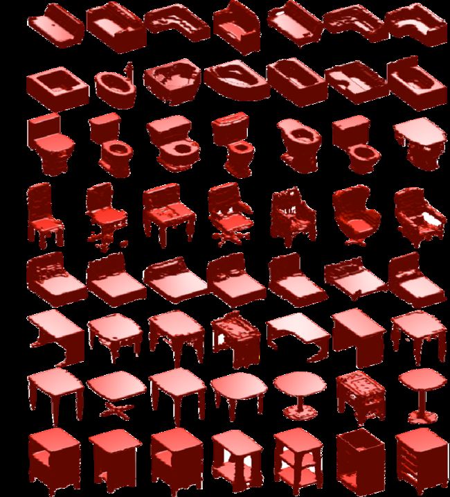
  第一种方法出自Princeton大学CVPR2015：《3D ShapeNets: A Deep Representation for Volumetric Shapes》，方法的核心是基于三维数据的“立体栅格化”，将Object的3D数据表示为 30×30∗30 大小的“立体栅格”，如下图：

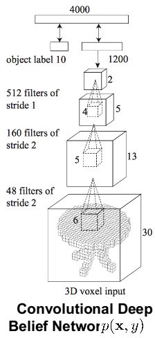
  之后，就在三维栅格数据上进行卷积网络的训练，网络结构图如下：



  第二种方法出自Massachusetts大学的ICCV2015：《Multi-view Convolutional Neural Networks for 3D Shape Recognition》。该方法主要对物体的三维数据，从不同的视角“拍摄”得到该物体的不同视角下的图像，将这些产生的二维图像作为训练数据。中间会有个“View Pooling”，接着会进行第二部分的卷积。如下：



  这两种方法产生的结果差异较大，于是作者就想应该是Volumetric CNN还没有充分的“挖掘”出3D representation的优势。
  这篇文章提出了两种“distinct network architecture of volumetric CNN”，提高了立体栅格CNN的效果。对于multiview CNNs，还提出了“multi-resolution filtering in 3D”，经过改造后的两种方法都取得了state-of-art的效果。

Introduction

  将2D卷积神经网络拓展，用于处理3D数据时，会有两个问题：
  1.additional computational complexity，3D数据的计算量将会极大的增加，就是所谓的“curse of dimensionality（维数灾难）”.

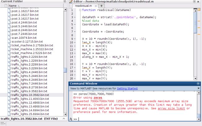
昨天我“立体栅格化”一个点云文件，有近7000个点，我在matlab里创建zeros(7000, 7000, 7000)，根本创建不了：

  2.data sparsity，数据的稀疏性。在一个立体网格中，点云只占了很小的一部分，其余部分都是0。这在昨天我在立体栅格化数据时，深有体会。

In this work, we analyze these observations and evaluate the design choices. Moreover, we show how to reduce the gap between volumetric CNNs and multi-view CNNs by efficiently augmenting training data, introducing new CNN architectures in 3D. Finally, we examine multi-view CNNs; our experiments show that we are able to improve upon state of the art with improved training data augmentation and a new multi-resolution component.

  这篇文章的工作：
  1.分析3D CNN为什么没能充分的“挖掘”三维形状信息，评价网络架构的设计；
  2.怎么减少3D CNN与Multi-view CNN之间的差距，通过增加训练数据，引入新的3D CNN结构；
  3.最后，测试Multi-view CNN，通过增加训练样本（improved training data augmentation），以及增加新的多分辨率的部分，来提高Multi-view CNN的结果。

Problem Statement，要解决的问题是什么？

  文章里说道：

We consider volumetric representations of 3D point clouds or meshes as input to the 3D object classification problem.

  3D object classification是以三维点云的立体表示作为输入数据的分类问题。这是因为实时的扫描数据是用立体的方式表示数据的。


  同时假设输入数据已经用3D bounding boxes预分割过了。

We further assume that the input data is already pre-segmented by 3D bounding boxes.

所谓的预分割，就是将原先总的点云数据，分割成一个个的instance（实例）：

  我们的任务就是，对这些实例进行分类，输出结果为立体数据的类别标签。

Approach

  提出了两种Volumetric CNN network architecture，这两种结构均在3D shape classification中，取得了state-of-art的效果，并且缩小了与Multi-view CNNs结构的差距：

The first network introduces auxiliary learning tasks by classifying part of an object, which help to scrutize details of 3D objects more deeply.

The second network uses long anisotropic kernels to probe for long-distance interactions.

  第一种网络方法很好理解，就是进一步解构出每个instance的细节，通过这些增加的更细节的数据来提高分类效果。第二种，long anisotropic kernels，我查阅资料，解释为“各向异性核函数”。不是很懂，先放一下。

We also conduct extensive experiments to study the influence of volume resolution, which sheds light on future
directions of improving volumetric CNNs.

  作者还研究了Volume的分辨率对实验结果的影响，这将为以后进一步提高Volume CNN指明方向。因为 30×30×30 的分辨率太低了，这大大影响了Volume CNN的表现。


  作者此外也进一步提高了Multi-view CNNs方法，引入了多分辨率的成分。

Furthermore, we introduce a new multi-resolution component to multi-view CNNs, which improves their already compelling performance.

  除了在3D CAD model datasets上做了大量的实验外，作者还在3D重建出的real-world 3D data上做了实验，用了M. Nießner et al.提出的3D重建方法。也比之前的方法能更好的适应从synthetic data（人工数据）到real-world data（真是世界的数据）。

Related Work

Analysis of state-of-the-art 3D Volumetric CNN versus Multi-View CNN

Two representations of generic 3D shapes are popularly used for object classification, volumetric and multi-view (Fig 1). The volumetric representation encodes a 3D shape as a 3D tensor of binary or real values. The multi-view representation encodes a 3D shape as a collection of renderings from multiple viewpoints. Stored as tensors, both representations can easily be used to train convolutional neural networks, i.e., volumetric CNNs and multi-view CNNs.

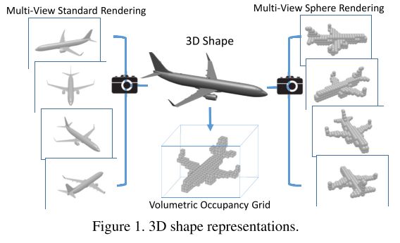
  现在流行的两种3D形状分类方法：volumetric CNNs、multi-view CNNs.
  volumetric representation：将3D形状转化为由二元值（0,1）或者实值表示的3D tensor.
  multi-view representation：将3D形状转化为一系列的多视角“拍摄”的2D 渲染图.
  由于是以tensor（多维数组）结构存储，因此两种表示都可以用CNN网络训练模型，如volumetric CNNs，以及multi-view CNNs.

Intuitively, a volumetric representation should encode as much information, if not more, than its multi-view counterpart. However, experiments indicate that multi-view CNNs produce superior performance in object classification. Fig 2 reports the classification accuracy on the ModelNet40 dataset by state-of-the-art volumetric multiview architectures1 . A volumetric CNN based on voxel occupancy (green) is 7.3% worse than a multi-view CNN (yellow).

  直观上，volumetric representation应该能够encode 3D形状很多的特征信息，至少不亚于multi-view representation。但是从实验结果来看，multi-view CNNs的结果远超于volumetric representation的方法。图2显示了目前最新的3D CNNs: 3D ShapeNet在ModelNet40数据集上的分类精度，基于立体栅格的3D CNNs的结果比multi-view CNNs的结果低出7.3%！（作者重现了3D ShapeNets、Multi-view CNNs的实验，并得出的精度评价.）

We investigate this performance gap in order to ascertain how to improve volumetric CNNs. The gap seems to be caused by two factors: input resolution and network architecture differences. The multi-view CNN downsamples each rendered view to 227 × 227 pixels (Multi-view Standard Rendering in Fig 1); to maintain a similar computational cost, the volumetric CNN uses a 30×30×30 occupancy grid (Volumetric Occupancy Grid in Fig 1 )2 . As shown in Fig 1, the input to the multi-view CNN captures more detail.

  作者就猜想这两者之间的差距可能来源于两个因素：输入数据的分辨率（input resolution），以及网络架构的差异（network architecture difference）。
Multi-view CNN将2D多视角渲染图像降采样到 227×227 ；为了保证计算效率，volumetric CNN用了 30×30×30 的立体栅格。图1就可以看出，multi-view的表示方法能捕获更多3D形状的细节信息。

However, the difference in input resolution is not the primary reason for this performance gap, as evidenced by further experiments. We compare the two networks by providing them with data containing similar level of detail. To this end, we feed the multi-view CNN with renderings of the 30×30×30 occupancy grid using sphere rendering3 , i.e., for each occupied voxel, a ball is placed at its center, with radius equal to the edge length of a voxel (Multi-View Sphere Rendering in Fig 1). We train the multi-view CNN from scratch using these sphere renderings. The accuracy of this multi-view CNN is reported in blue.

  但是，输入数据分辨率的差距并不是两者表现之间差距的首要原因，这点会在后面的实验证明。
  因为我们输入两个网络进相等水平的细节信息。为了达到提供两个网络相似细节信息的目的，我们给multi-view CNN网络提供的数据，是来自于 30×30×30 立体栅格，通过对这个栅格不同的视角“拍摄”得到的。这个立体栅格每个voxel填充的是ball，一个球。（至于为什么不把立体栅格的分辨率上升到 227×227×227 ，这样，volumetric representation的细节信息，就能够与 227×227 的渲染图同水平了。不这样做的原因是考虑计算代价， 2273 太大了，计算量太大，就这是前面所说的“数为灾难”）
  这种输入数据，multi-view CNNs得到的分类精度如表中蓝色线所示。可以发现，蓝色线89.5%的分类精度还是远比3D ShapeNets的分类精度84.7%高出很多。

As shown in Fig 2, even with similar level of object detail, the volumetric CNN (green) is 4.8% worse than the multi-view CNN (blue). That is, there is still significant room to improve the architecture of volumetric CNNs. This discovery motivates our efforts in Sec 4 to improve volumetric CNNs. Additionally, low-frequency information in 3D seems to be quite discriminative for object classification—it is possible to achieve 89.5% accuracy(blue) at a resolution of only 30×30×30. This discovery motivates our efforts in Sec 5 to improve multi-view CNNs with a 3D multi-resolution approach.

  根据上面的实验，即使降低输入数据的细节信息，multi-view的分类精度还是比同等细节信息下的3D ShapeNets高出4.8%。所以，volumetric CNNs架构还有很大的提升空间。
  另外，这个降低细节信息给multi-view CNNs的实验，都达到了89.5%的分类精度，这个发现提示了我们用多分辨率的3D模型来提升multi-view CNNs的工作。

Volumetric Convolutional Neural Networks

Overview

We improve volumetric CNNs through three separate means: 1) introducing new network structures; 2) data augmentation; 3) feature pooling.

  作者为了提升volumetric CNNs的分类精度，从3个独立的方法分别进行了尝试实验：
  （1）引入新的卷积网络结构；
  （2）进行训练数据的增加（data augmentation）；
  （3）特征池化。

Network Architecture

We propose two network variations that significantly improve state-of-the-art CNNs on 3D volumetric data. The first network is designed to mitigate overfitting by introducing auxiliary training tasks, which are themselves challenging. These auxiliary tasks encourage the network to predict object class labels from partial subvolumes. Therefore, no additional annotation efforts are needed. The second network is designed to mimic multi-view CNNs, as they are strong in 3D shape classification. Instead of using rendering routines from computer graphics, our network projects a 3D shape to 2D by convolving its 3D volume with an anisotropic probing kernel. This kernel is capable of encoding long-range interactions between points. An image CNN is then appended to classify the 2D projection. Note that the training of the projection module and the image classification module is end-to-end. This emulation of multi-view CNNs achieves similar performance to them, using only standard layers in CNN.

  提出两种网络，可以有效的提升现在state-of-art CNNs在volumetric data上的效果。
  第一个网络，是引入辅助的训练任务来减小过拟合，这种辅助任务是使用部分的立体数据（partial subvolumes）来预测物体的类别。仅仅是一部分的立体数据，所以也不需要额外的任务。
  第二个网络是模仿multi-view CNNs，不过数据不是由不同路径“拍摄”得到的多视角二维渲染图（这部分请看论文《Multi-view CNNs》），而是将3D形状数据通过与一个各向异性“探索”核进行卷积，将3D数据投影到2D数据上。这种各向异性核函数能够把长距离的点进行“encoding”，之后一个2D图像的卷积网络用来对这些投影后的2D图像进行分类。注意到，投影模型、分类模型的训练是端到端的。
  关于“anisotropic kernel”我没有见过，我查了很多资料，但是仍理不清。后来问了小虎师兄，他大概跟我讲了一下。所谓的各向异性核（想象成卷积中的卷积核），是与各向同性核类似，各向同性核是“radially symmetry”，镜像对称的，卷积核中在一个点的位置只与到中心点的距离有关，而与该点的方向无关。而各向异性核，类似于椭圆，椭球，就与一个点处的值，就与方向有关了。其实网上的“anisotropic kernel”资料不少，但大多是论文中的资料，没有基础看的是一头雾水。我也是定性的理解了一下，推荐一篇论文：《Image and Video Segmentation by Anisotropic Kernel Mean Shift》，ECCV2004年的，这篇论文讲的“anisotropic kernel”还挺好。有时间弄懂了细讲。
  还有这里，所谓的“anisotropic probing kernel”，“各项异性探索核”，我想指的是这种核是要通过CNN来训练得到吧，后一句也提到了，这种训练是端到端的，因此，我想这里的“probing”，是这么个意思。
  这种仿效multi-view CNNs的做法取得了与之类似的效果，也只用了标准的CNN层。

In order to mitigate overfitting from too many parameters, we adopt the mlpconv layer from [23] as our basic building block in both network variations.

  为了减少参数过多容易造成了过拟合问题，我们采用文献[23]的《Nerwork in Network, NIN》mplconv layer作为我们网络的基础构件。

Data Augmentation

Compared with 2D image datasets, currently available 3D shape datasets are limited in scale and variation. To fully exploit the design of our networks, we augment the training data with different azimuth and elevation rotations. This allows the first network to cover local regions at different orientations, and the second network to relate distant points at different relative angles.

  进行数据的曾广，将训练数据从不同方向、不同高度旋转等操作。

Multi-orientation Pooling

Both of our new networks are sensitive to shape orientation, i.e., they capture different information at different orientations. To capture a more holistic sense of a 3D object, we add an orientation pooling stage that aggregates information from different orientations.

  由于从不同的方向获取不同的信息，我们的CNN网络对物体的方向是“sensitive”，敏感的。因此，我们增加一个方向池化阶段，将不同方向的信息进行pooling，以取得类似于方向不变性的性质。

Network 1: Auxiliary Training by Subvolume Supervision

We observe significant overfitting when we train the volumetric CNN proposed by [33] in an end-to-end fashion (see supplementary). We thus introduce auxiliary tasks that are closely correlated with the main task but are difficult to overfit, so that learning continues even if our main task is overfitted.

  Princeton大学的Wu提出的3D ShapeNet，作者在训练这个3D ShapeNet的时候，发现明显的过拟合现象。
因此，作者引入了一个新的辅助训练任务，很难过拟合。即使主任务过拟合了，由于辅助任务很难过拟合，因此，训练还可以继续。否则单一的主任务，一旦过拟合，训练就停止了。

These auxiliary training tasks also predict the same object labels, but the predictions are made solely on a local subvolume of the input. Without complete knowledge of the object, the auxiliary tasks are more challenging, and can thus better exploit the discriminative power of local regions.

  引入的辅助任务就是用局部的3D形状数据来预测整体的类别，这个任务是很难的。因为是用部分来预测整体。也能更好的挖掘每个形状局部的特征信息。

We implement this design through an architecture shown in Fig 3. The first three layers are mlpconv (multilayer perceptron convolution) layers, a 3D extension of the 2D mlpconv proposed by [23]. The input and output of our mlpconv layers are both 4D tensors. Compared with the standard combination of linear convolutional layers and max pooling layers, mlpconv has a three-layer structure and is thus a universal function approximator if enough neurons are provided in its intermediate layers. Therefore, mlpconv is a powerful filter for feature extraction of local patches, enhancing approximation of more abstract representations. In addition, mlpconv has been validated to be more discriminative with fewer parameters than ordinary convolution with pooling [23].

At the fourth layer, the network branches into two. The lower branch takes the whole object as input for traditional classification. The upper branch is a novel branch for auxiliary tasks. It slices the 512 × 2 × 2 × 2 4D tensor (2 grids along x, y, z axes and 512 channels) into 2×2×2 = 8 vectors of dimension 512. We set up a classification task for each vector. A fully connected layer and a softmax layer are then appended independently to each vector to construct classification losses. Simple calculation shows that the receptive field of each task is 22×22×22, covering roughly 2/3 of the entire volume.

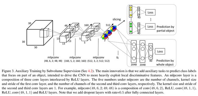
  图3是 第一种引入辅助任务的网络结构示意图。
  网络的头3层是mlpconv（multilayer perceptron convolution）层，这是文献23《Network in Network，NIN》中提出的mlpconv层从2D到3D的扩展。我们的mlpconv层的输入与输出都是4D tensor。相比较于标准的卷积层与池化层的组合，mlpconv层 有三层结构，如果在mlpconv层的中间有足够多的神经元的，它可以拟合几乎所有的函数。因此，mlpconv结构对于局部区域（local patch）特征的提取十分有效。还有，mlpconv结构比原来的convolution层加上pooling层有着少的参数。

  在第四层，我们的网络结构分为两个分支。下面的分支输入进的是整个3D形状数据，来做经典的分类任务。
上面的分支是上述新加的辅助任务的分支，它将 512×2×2×2 这4D tensor（沿着 x,y,z轴 各2个“格子”，512个channels，看图中彩色方块，就是512个方块，每个方块的 x,y,z 轴各有2个小格子），切分成 2×2×2=8 个512维向量。
  slice，切分的方法是，从每个方块的 x,y,z 坐标来看，坐标 (x,y,z)=(1,1,1) 的位置，共512个，这个组成一个vector；同理，512个方块上，相同坐标 (1,1,2),(1,2,1),(1,2,2),(2,1,1),(2,1,2),(2,2,1),(2,2,2) 的位置被“slice”成一个vector，共8个这样的vector。
  我们对每个vector（512 dim）进行分类一个分类任务。随后每个向量后面各自加上一个fully connected layer（40个neurons，每个neuron代表一个class），以及softmax layer，来计算分类的loss。
  由于上面的网络，是将特征分开来，每个部分（图中是8个部分）独立的预测整体的类别。最后那句：“Simple calculation shows that the receptive field of each task is 22×22×22”，我琢磨了好久，这里解释下：
  原先，每经过一层卷积后的维数是这么算的：
  第一层mlpconv： 30−62+1=13 ，第一层mlpconv中间还有两个网中网的卷积，但由于卷积核、卷积的步长都是1，所以卷积后的大小仍是13，没有变，以下同理。
  第二层mlpconv： 13−52+1=5 ，
  第三层mlpconv： 5−32+1=2 .
  由于只使用了 2×2×2 方块中的每1块来独立地预测。因此，这个“每1块”反推回去得到的方块大小，就是最开始使用的实际大小。因此，将1块：
  

x−32+1=1

  得到： x=3

  

x−52+1=3

  得到： x=9
  

x−62+1=9

  解得：

x=22

  故，辅助任务部分，实际上使用的原始大小为 22×22×22 个部分格子，原始总共 30×30×30 大小，故实现了 一部分预测整体。

Network 2: Anisotropic Probing

The success of multi-view CNNs is intriguing. multi-view CNNs first project 3D objects to 2D and then make use of well-developed 2D image CNNs for classification. Inspired by its success, we design a neural network architecture that is also composed of the two stages. However, while multi-view CNNs use external rendering pipelines from computer graphics, we achieve the 3D-to-2D projection using network layers in a manner similar to ‘X-ray scanning’.

  受到Multi-view CNNs成功的启发，我们设计了一个也由两个阶段组成的网络结构。但是，Multi-view CNNs是将3D形状物体通过计算机进行渲染，得到3D渲染图，之后，通过规定的“路线”，“摄像机”沿着这个“路线”“拍摄”得到多视角2D图像。然而，我们从3D到2D的投影图用神经网络以类似于“X-ray 扫描”的方式获取的。

Key to this network is the use of an elongated anisotropic kernel which helps capture the global structure of the 3D volume. As illustrated in Fig 4, the neural network has two modules: an anisotropic probing module and a network in network module. The anisotropic probing module contains three convolutional layers of elongated kernels, each followed by a nonlinear ReLU layer. Note that both the input and output of each layer are 3D tensors.

  网络的关键是用一个拉长的各向异性核来获取3D形状的全局结构。
  如图4所示，我们的这个网络有两个模块，各向异性核探测模块，以及Network in Network模块。各向异性核探索模块包含3个被拉长的核的卷积层，每一个后面照例会有一个ReLU层。注意，每一层的输入输出都是3D tensor。

In contrast to traditional isotropic kernels, an anisotropic probing module has the advantage of aggregating long-range interactions in the early feature learning stage with fewer parameters. As a comparison, with traditional neural networks constructed from isotropic kernels, introducing long-range interactions at an early stage can only be achieved through large kernels, which inevitably introduce many more parameters. After anisotropic probing, we use an adapted NIN network [23] to address the classification problem.

  相比较与传统的各向同性核，各向异性探索核模块在早期的特征学习阶段可以用更少的参数来聚集长距离的关系特征。相比较于传统的各向同性核，若想结合长距离的关系特征，就得用更大的核，而更大的核肯定会带来更多的参数。在各向异性探索模块之后，我们用一个调整好的NIN网络来处理分类问题。

Our anistropic probing network is capable of capturing internal structures of objects through its X-ray like projection mechanism. This is an ability not offered by standard rendering. Combined with multi-orientation pooling (introduced below), it is possible for this probing mechanism to capture any 3D structure, due to its relationship with the Radon transform.

In addition, this architecture is scalable to higher resolutions, since all its layers can be viewed as 2D. While 3D convolution involves computation at locations of cubic resolution, we maintain quadratic compute.

  我们的各向异性核模块，类似于X-ray的“穿透机制”，能够“穿透”3D物体，捕获内部的结构特征信息，提取到标准渲染图方式提取不到的信息。结合下面要讲的多方向池化（multi-orientation pooling），由于对数据进行了随见变换，我们可以提取到任何的3D结构特征。
  除此之外，我们的架构可以延展到更高的分辨率，因为它的所有层可以视为2D的。当3D卷积的消耗时间与立方体的分辨率有关，我们保证二次方的计算。（这地方不是很懂，但感觉对主干理解没太大影响，先略去。）

Data Augmentation and Multi-Orientation Pooling

  这一部分就是数据增广，以及多方向池化。
  以上两个网络，都对数据数据的方向是敏感的。在第一个辅助任务的网络中，不同的数据模型方向就对应了不同的subvolume；在第二个各向异性网络中，只有与各向异性核的长轴方向一致的voxels可以通过各向异性核进行长距离的特征的交互提取。因此，将训练数据从各个方向进行增广操作，从各个方向提取特征，并通过多方向池化来进行结合。这样来获取方向不变性的特性。

Similar to Su-MVCNN [32] which aggregates information from multiple view inputs through a view-pooling layer and follow-on fully connected layers, we sample 3D input from different orientations and aggregate them in a multi-orientation volumetric CNN (MO-VCNN) as shown in Fig 5.

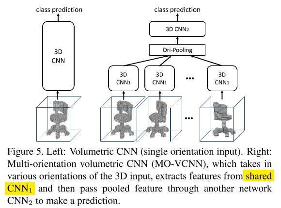
  与Su的MVCNN网络从各个视角提取信息再通过view-pooling层以及随后的fully-connected层进行特征的聚合类似，我们从不同的方向提取3D形状特征信息，再将它们聚合在multi-orientation volumetric CNN中，如图5所示。

At training time, we generate different rotations of the 3D model by changing both azimuth and elevation angles, sampled randomly. A volumetric CNN is firstly trained on single rotations. Then we decompose the network to CNN1 (lower layers) and CNN2 (higher layers) to construct a multi-orientation version.

The MO-VCNN’s weights are initialized by a previously trained volumetric CNN with CNN1’s weights fixed during fine-tuning.

While a common practice is to extract the highest level features (features before the last classification linear layer) of multiple orientations, average/max/concatenate them, and train a linear SVM on the combined feature, this is just a special case of the MO-VCNN.

  在训练阶段，我们通过同时地随机改变方向角、高度角来生成不同旋转角度的3Dmodel。每一个不同旋转角度的3D模型先在一个volumetric CNN上训练。我们将网络分解为CNN1*（低层部分）和CNN2（高层部分）来建立一个多方向的volumetric CNN。
  MOVCNN的权重是由之前训练好的volumetric CNN来提供的，同时，MOVCNN的低层部分，即CNN1部分的权重在微调的时候是固定的。
  一个常见的操作是，在提取多方向的高层特征后（就是在最后的线性分类层之前的特征），进行average或max或concatenate操作，然后用一个线性的SVM来训练这些多方向结合的特征，这只是MO-VCNN中的一个特例。

Compared to 3DShapeNets [33] which only augments data by rotating around vertical axis, our experiment shows that orientation pooling combined with elevation rotation can greatly increase performance.

  3D ShapeNets只通过围绕3D Shape的垂直轴旋转来进行数据增广，相比之下，我们的实验显示结合高度角的旋转增广操作提取到的特征，可以使结果有很大的提高。

Multi-view Convolution Neural Network

The multi-view CNN proposed by [32] is a strong alternative to volumetric representations. This multi-view representation is constructed in three steps: first, a 3D shape is rendered into multiple images using varying camera extrinsics; then image features (e.g. conv5 feature in VGG or AlexNet) are extracted for each view; lastly features are combined across views through a pooling layer, followed by fully connected layers.

  Multi-view CNN是volumetric representation的另一种强有力的替代方法。Multi-view representation有以下三步：
  （1）根据相机外参数得到3D渲染，再得到不同视角的图像。
  （2）用卷积网络来提取每一张图像的特征；
  （3）最后经过一个pooling层进行特征的融合，随后就是fully connected layer。

Although the multi-view CNN presented by [32] produces compelling results, we are able to improve its performance through a multi-resolution extension with improved data augmentation.

We introduce multi-resolution 3D filtering to capture information at multiple scales. We perform sphere rendering (see Sec 3) at different volume resolutions. Note that we use spheres for this discretization as they are view-invariant. In particular, this helps regularize out potential noise or irregularities in real-world scanned data (relative to synthetic training data), enabling robust performance on real-world scans.

Note that our 3D multi-resolution filtering is different from classical 2D multi-resolution approaches, since the 3D filtering respects the distance in 3D.

  尽管Multi-view CNNs已经取得了很好的效果，但是我们仍可以通过多分辨率来进行数据增广，以此提高结果。
  我们引入一个多分辨率的3D filtering来提取不同尺度下的特征信息。
  我们对不同分辨率下的volume实施球形渲染（sphere rendering），就是在每个voxel中用“圆球”填充，代替原先的方格。我们用球形渲染的原因是它们是与视点无关的（view-invariant）。特别是，这可以帮助我们regularize out真实世界扫描的数据中潜在的noise，以及irregularities，使得在处理真实世界数据是更加robust。
  要注意我们的3D multi-resolution filtering不同于经典的2D multi-resolution方法，因为3D filtering与3D中的距离有关。（sorry，是在不知道怎么翻译…就直接用英文吧，意思反而更准确些…）

Experiments

We evaluate our volumetric CNNs and multi-view CNNs along with current state of the art on the ModelNet dataset [33] and a new dataset of real-world reconstructions of 3D objects.

  我们测试评估volumetric CNNs、multi-view CNNs沿用现今最新的ModelNets数据集，以及一个新的真实世界3D 物体重建的数据集。

Datasets

ModelNet

We use ModelNet [33] for our training and testing datasets. ModelNet currently contains 127, 915 3D CAD models from 662 categories. ModelNet40, a subset including 12, 311 models from 40 categories, is well annotated and can be downloaded from the web. The authors also provide a training and testing split on the website, in which there are 9, 843 training and 2, 468 test models4 . We use this train/test split for our experiments.

  我们使用ModelNet数据集来训练测试。ModelNet现今有 127,915 张3D CAD模型（来自 662 个类别）。ModelNet40，是其中一个包含 12,311 张模型（ 40 个类别）的子数据集。作者也提供了将训练集、测试集分开的数据集，训练集共有 9,843 张模型，测试集有 2,468 个模型。我们用这个训练/测试分类来做实验。

By default, we report classification accuracy on all models in the test set (average instance accuracy). For comparisons with previous work we also report average class accuracy.

  默认情况下，我们报告所有模型的分类精度是测试集上的（average instance accuracy，平均实例精度）。为了与之前工作对比，我们还报告平均类别精度（average class accuracy）。

Real-world Reconstructions

We provide a new real-world scanning dataset benchmark, comprising 243 objects of 12 categories; the geometry is captured with an ASUS Xtion Pro and a dense reconstruction is obtained using the publicly-available VoxelHashing framework [25]. For each scan, we have performed a coarse, manual segmentation of the object of interest. In addition, each scan is aligned with the world-up vector.

While there are existing datasets captured with commodity range sensors – e.g., [29, 34, 31] – this is the first containing hundreds of annotated models from dense 3D reconstructions. The goal of this dataset is to provide an example of modern real-time 3D reconstructions; i.e., structured representations more complete than a single RGB-D frame but still with many occlusions. This dataset is used as a test set.

  提供一个真实世界扫描数据标准集，包括243个物体，12个类别；物体的几何形状是由ASUS Xtion Pro采集的，重建是用文献[25]提供的开源的VoxelHashing framework。对于每一个扫描，我们对感兴趣物体进行了一个粗糙的人工分割。除此之外，In addition, each scan is aligned with the world-up vector.，这句不明白。
  尽管也存在其他的数据集了，如[29, 34, 31]，但这是第一个包含上百张标注好的模型3D重建模型。这个数据集的目的是为了提供一个现代实时3维重建的例子；这个数据集是用来测试的。

Comparison with State-of-the-Art Methods

Volumetric CNNs

Fig 7 summarizes the performance of volumetric CNNs. Ours-MO-SubvolumeSup is the subvolume supervision network in Sec 4.2 and Ours-MO-AniProbing is the anistropic probing network in Sec 4.3. Data augmentation is applied as described in Sec 6.4 (azimuth and elevation rotations). For clarity, we use MO- to denote that both networks are trained with an additional multi-orientation pooling step (20 orientations in practice). For reference of multi-view CNN performance at the same 3D resolution, we also include Ours-MVCNN-Sphere-30, the result of our multi-view CNN with sphere rendering at 3D resolution 30. More details of setup can be found in the supplementary.

As can be seen, both of our proposed volumetric CNNs significantly outperform state-of-the-art volumetric CNNs. Moreover, they both match the performance of our multi- view CNN under the same 3D resolution. That is, the gap between volumetric CNNs and multi-view CNNs is closed under 3D resolution 30 on ModelNet40 dataset, an issue that motivates our study (Sec 3).

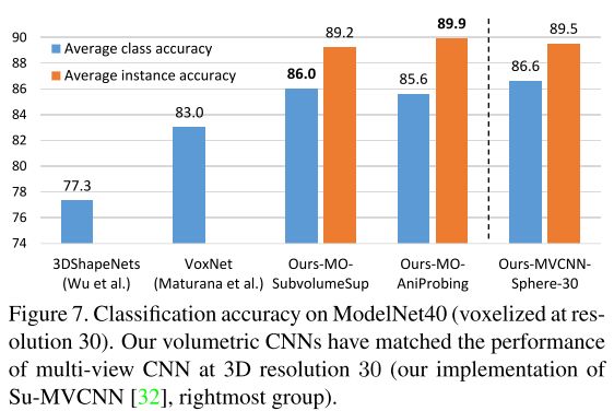
  这一部分就是实验，主要是在ModelNet40数据集上做实验，分为两部分，一部分是Volumetric CNNs的方法，另一部分是提升Multi-view CNNs的方法。
先说Volumetric CNNs的方法，作者在上面提出了两种改进网络：一种是文章4.2提出的Network 1: Auxiliary Training by Subvolume Supervision，即用部分预测整体。网络结构我用Graphviz画出来了，如下（限于篇幅，我截取了最后一部分）：

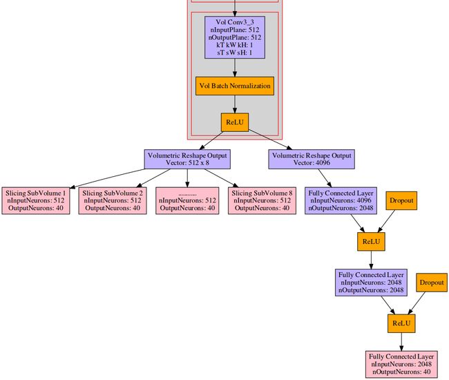
  我想上面的结构图比论文中的要好懂多了，结构更清晰。
  另一种 “Anisotropic Probing Kernel”，即各向异性核函数的方法，网络结构如下：

  实际我在跑作者提供的源代码的时候，作者还写了一个网络结构： 3D_NIN _FC，即在3层NIN网络后面直接用Fully Connected Layer层。这应该算是很经典的一种结构吧，就是卷积之后来个全连接进行分类。
  我跑了这这个网络model，预训练是在 modelnet40_60x数据上，这部分数据 include azimuth and elevation rotation augmented occupancy grids，即既做了方位角上的 Data Augmentation，也做了高度角上的 Data Augmentation，最后预训练的 Mean Class Accuracy ：

  预训练达到的最高精度是 83.779038357645%。
  预训练完成后，进行 fine-tuning，fine-tuning是在 modelnet40_20x_stack数据集上，这个数据集是用于多方向训练的。fine-tuning后， Mean Class Accuracy曲线如下：

   3D_NIN_FC在测试集上fine-tuning后的最高精度是： 90.032414910859%。 训练用时48h，fine-tuning用时半小时就搞定了。
  在 subvolume_sup.lua、aniprobing.lua的模型还在训练中…
  给出作者自己的训练结果：

Multi-view CNNs

Fig 8 summarizes the performance of multi-view CNNs. Ours-MVCNN-MultiRes is the result by training an SVM over the concatenation of fc7 features from Ours-MVCNN-Sphere-30, 60, and Ours-MVCNN. HoGPyramid-LFD is the result by training an SVM over a concatenation of HoG features at three 2D resolutions. Here LFD (lightfield descriptor) simply refers to extracting features from renderings. Ours-MVCNN-MultiRes achieves state-of-the-art.

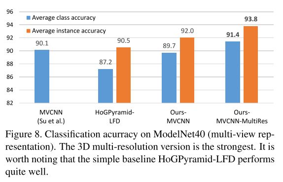
  这部分的实验作者没有提供 torch源码，反而提供了 caffe的 multiview_deploy.prototxt，有待训练。
  这部分的 Ours-MVCNN-MultiRes是用CNN提取 Sphere-30, 60多分辨率的特征后，放入SVM进行训练得到的结果。 Ours-MVCNN、HoGPyramid-LFD是通过HoG提取多分辨率特征，再在SVM上训练。 LFD（LightField Descriptor）指的是从rendering中提取特征。

Effect of 3D Resolution over Performance

Fig 9 shows the performance of our volumetric CNN and multi-view CNN at different 3D resolutions (defined at the beginning of Sec 6). Due to computational cost, we only test our volumetric CNN at 3D resolutions 10 and 30.

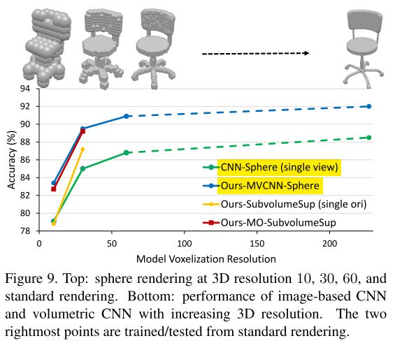
The observations are:
first, the performance of our volumetric CNN and multi-view CNN is on par at tested 3D resolutions;

second, the performance of multi-view CNN increases as the 3D resolution grows up. To further improve the performance of volumetric CNN, this experiment suggests that it is worth exploring how to scale volumetric CNN to higher 3D resolutions.

  这一部分作者对不同分辨率下的3D数据，对Volumetric CNNs与Multi-view CNNs的影响进行了讨论研究。由于计算能力的限制，对于Volumetric CNNs的部分，数据的分辨率只有10与30。
  发现了两点：
  （1）在在同等的分辨率下，多视角数据训练后，深蓝色的Ours-MVCNN-Sphere的表现与Ours-MO-Subvolumesup的表现一致；单视角的CNN-Sphere(single view)与Ours-SubvolumeSup(single ori)表现也基本一致。只不过看图中，在30分辨率下的黄色的Ours-SubvolumeSup(single ori)结果要好于CNN-Sphere(single view)。
  （2）第二点观察到的结论就是，分辨率越高，结果越好。因此，若能将Volumetric CNNs用于处理更高分辨率的数据，会有更好的效果。因此，这个方向进行研究是很有意义的。