python批量处理海面温度(.nc)数据
新手初学python,想用博客记录一下,欢迎和大家共同学习
对于海面温度数据,下载地址ERA5-Land hourly data from 1981 to present (copernicus.eu)
绘制区域地图,参考此篇博客(3条消息) 利用Cartopy库绘制地图_x5675602的专栏-CSDN博客
#引入所需要的包
import numpy as np
import matplotlib.pyplot as plt
import cartopy.crs as ccrs
import cartopy.feature as cfeature
from cartopy.mpl.ticker import LongitudeFormatter, LatitudeFormatter
import netCDF4 as nc
#读取单个nc文件
f1 = nc.Dataset(r'F:\project\nc\data-sst\adaptor.mars.internal-SST2018.nc')
# print(f1) #可以了解f1有哪些内容
#将f1里面的变量存储到等号左边
lat = f1.variables['latitude'][:]
lon = f1.variables['longitude'][:]
time = f1.variables['time'][:]
sst = f1.variables['sst'][:]
data_sst = sst[0,:,:]-273.15
box = [100, 150, 0, 50]#根据自己的研究区域确定经纬度
scale = '50m'
xstep, ystep = 10, 10
fig = plt.figure(figsize=(8, 10))
ax = plt.axes(projection=ccrs.PlateCarree())
# set_extent需要配置相应的crs,否则出来的地图范围不准确
ax.set_extent(box, crs=ccrs.PlateCarree())
land = cfeature.NaturalEarthFeature('physical', 'land', scale, edgecolor='face',
facecolor=cfeature.COLORS['land'])
ax.add_feature(land, facecolor='0.75')
ax.coastlines(scale)
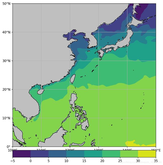
sst = plt.contourf(lon,lat,data_sst)#这里是画温度图
ax.set_xticks(np.arange(box[0], box[1]+xstep,xstep), crs=ccrs.PlateCarree())
ax.set_yticks(np.arange(box[2], box[3]+ystep,ystep), crs=ccrs.PlateCarree())
# zero_direction_label用来设置经度的0度加不加E和W
lon_formatter = LongitudeFormatter(zero_direction_label=False)
lat_formatter = LatitudeFormatter()
ax.xaxis.set_major_formatter(lon_formatter)
ax.yaxis.set_major_formatter(lat_formatter)
# 添加网格线
ax.grid()
plt.colorbar(location='bottom', fraction=0.05, pad=0.02)#添加色标
plt.show()
结果图
对于如何批量读取sst数据,需要写一个循环进行调用即可
import numpy as np
import matplotlib.pyplot as plt
import cartopy.crs as ccrs
import cartopy.feature as cfeature
from cartopy.mpl.ticker import LongitudeFormatter, LatitudeFormatter
import netCDF4 as nc
import os


def readfiles(files):
    for f in files:
        f1 = nc.Dataset(f)
        lat = f1.variables['latitude'][:]
        lon = f1.variables['longitude'][:]
        time = f1.variables['time'][:]
        sst = f1.variables['sst'][:]
        data_sst = sst[0,:,:]-273.15

        box = [100, 150, 0, 50]
        scale = '50m'
        xstep, ystep = 10, 10
        fig = plt.figure(figsize=(8, 10))
        ax = plt.axes(projection=ccrs.PlateCarree())
        # set_extent需要配置相应的crs,否则出来的地图范围不准确
        ax.set_extent(box, crs=ccrs.PlateCarree())
        land = cfeature.NaturalEarthFeature('physical', 'land', scale, edgecolor='face',
                                    facecolor=cfeature.COLORS['land'])
        ax.add_feature(land, facecolor='0.75')
        ax.coastlines(scale)

        sst = plt.contourf(lon,lat,data_sst)
        ax.stock_img()
        #标注坐标轴
        ax.set_xticks(np.arange(box[0], box[1]+xstep,xstep), crs=ccrs.PlateCarree())
        ax.set_yticks(np.arange(box[2], box[3]+ystep,ystep), crs=ccrs.PlateCarree())
        # zero_direction_label用来设置经度的0度加不加E和W
        lon_formatter = LongitudeFormatter(zero_direction_label=False)
        lat_formatter = LatitudeFormatter()
        ax.xaxis.set_major_formatter(lon_formatter)
        ax.yaxis.set_major_formatter(lat_formatter)
        # 添加网格线
        ax.grid()
        name_file = os.path.basename(f)
        out_path = r'F:\project\nc\data-sst-jpg'#此处为输出路径
        fname = os.path.join(out_path, name_file + '_front.jpg')#数据路径的jpg存储名称
        plt.colorbar(location='bottom', fraction=0.05, pad=0.02)#添加色标
        plt.savefig(fname=fname, dpi=150, bbox_inches='tight')#输出图像保存
        # print("sucessful")
        # plt.show()

file_path = r'F:\project\nc\data-sst'

file_list = os.listdir(file_path)
files = [os.path.join(file_path,x) for x in file_list]
file = readfiles(files)#调用readfiles函数