Naive Bayes 朴素贝叶斯代码实现-Python

Implementing Naive Bayes in Python

To actually implement the naive Bayes classifier model, we’re going to use scikit-learn, and we’ll import our GaussianNB from sklearn.naive_bayes.

import numpy as np
import pandas as pd
from sklearn.model_selection import train_test_split
from sklearn.naive_bayes import GaussianNB
from sklearn.metrics import accuracy_score
import matplotlib.pyplot as plt
import seaborn as sns

Load the Data

Once the libraries are imported, our next step is to load the data, stored in the GitHub repository linked here.

df = pd.read_csv('Naive-Bayes-Classification-Data.csv')
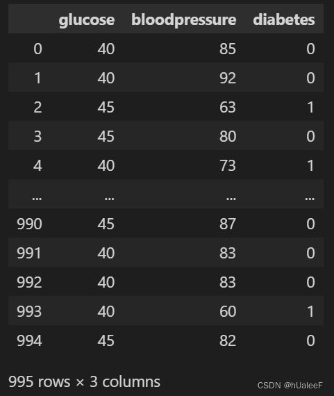
df

Also, in the snapshot of the data below.

Data pre-processing

Here, we’ll create the x and y variables by taking them from the dataset and using the train_test_split function of scikit-learn to split the data into training and test sets.

Note that the test size of 0.25 indicates we’ve used 25% of the data for testing. random_state ensures reproducibility. For the output of train_test_split, we get x_train, x_test, y_train, and y_test values.

x = df.drop('diabetes', axis=1)
y = df['diabetes']
x_train, x_test, y_train, y_test =train_test_split(x, y, test_size=0.25, random_state=42)

Train the model

We’re going to use x_train and y_train, obtained above, to train our naive Bayes classifier model. We’re using the fit method and passing the parameters as shown below.

model = GaussianNB()
model.fit(x_train, y_train)

Prediction

Once the model is trained, it’s ready to make predictions. We can use the predict method on the model and pass x_test as a parameter to get the output as y_pred.

Notice that the prediction output is an array of real numbers corresponding to the input array.

y_pred = model.predict(x_test)
y_pred

# output
array([1, 1, 1, 0, 0, 0, 1, 0, 0, 1, 0, 0, 0, 0, 0, 1, 1, 1, 1, 0, 0, 1,
       1, 0, 0, 0, 1, 1, 0, 0, 0, 1, 0, 1, 0, 1, 1, 0, 0, 0, 1, 0, 0, 0,
       0, 0, 1, 1, 1, 1, 0, 1, 0, 1, 1, 1, 1, 1, 1, 1, 0, 1, 1, 1, 0, 1,
       1, 0, 1, 1, 0, 0, 0, 0, 1, 1, 0, 0, 1, 1, 0, 0, 0, 0, 0, 0, 0, 1,
       0, 1, 0, 0, 1, 0, 1, 1, 0, 1, 1, 1, 1, 1, 1, 0, 0, 1, 1, 0, 1, 0,
       1, 0, 1, 0, 0, 1, 0, 0, 1, 1, 1, 0, 0, 0, 0, 1, 1, 0, 1, 1, 1, 0,
       0, 0, 1, 1, 1, 1, 0, 1, 1, 0, 1, 1, 1, 1, 0, 0, 1, 1, 0, 1, 0, 0,
       1, 1, 1, 0, 0, 1, 1, 1, 0, 1, 1, 1, 0, 0, 1, 1, 1, 0, 1, 0, 0, 1,
       0, 1, 1, 1, 1, 1, 0, 0, 0, 1, 1, 1, 0, 1, 1, 1, 1, 0, 0, 1, 0, 0,
       0, 0, 1, 1, 1, 1, 0, 1, 1, 1, 0, 0, 1, 1, 1, 1, 1, 1, 1, 1, 0, 0,
       1, 1, 0, 0, 1, 1, 1, 1, 0, 0, 1, 0, 0, 1, 0, 1, 1, 0, 1, 0, 1, 0,
       1, 0, 1, 0, 0, 0, 0])

Model Evaluation

Finally, we need to check to see how well our model is performing on the test data. For this, we evaluate our model by finding the accuracy score produced by the model.

accuracy = accuracy_score(y_test, y_pred)*100
accuracy

# output
92.7710843373494

References

1. Naive Bayes Classifier in Python Using Scikit-learn
2. Naive-Bayes data