Open AI 自监督学习笔记：Self-Supervised Learning | Tutorial | NeurIPS 2021

转载自微信公众号
原文链接： https://mp.weixin.qq.com/s?__biz=Mzg4MjgxMjgyMg==&mid=2247486049&idx=1&sn=1d98375dcbb9d0d68e8733f2dd0a2d40&chksm=cf51b898f826318ead24e414144235cfd516af4abb71190aeca42b1082bd606df6973eb963f0#rd

Open AI 自监督学习笔记

---

---

Video: https://www.youtube.com/watch?v=7l6fttRJzeU
Slides: https://nips.cc/media/neurips-2021/Slides/21895.pdf

Self-Supervised Learning
– Self-Prediction and Contrastive Learning

• Self-Supervised Learning
  • a popular paradigm of representation learning

Outline

• Introduction: motivation, basic concepts, examples
• Early Work: Look into connection with old methods
• Methods
  • Self-prediction
  • Contrastive Learning
  • (for each subsection, present the framework and categorization)
• Pretext tasks: a wide range of literature review
• Techniques: improve training efficiency

Introduction

What is self-supervised learning and why we need it?

What is self-supervised learning?

• Self-supervised learning (SSL):
  • a special type of representation learning that enables learning good data representation from unlablled dataset
• Motivation :

  • the idea of constructing supervised learning tasks out of unsupervised datasets

  • Why?

    ✅ Data labeling is expensive and thus high-quality dataset is limited

    ✅ Learning good representation makes it easier to transfer useful information to a variety of downstream tasks $\Rightarrow$ e.g. Few-shot learning / Zero-shot transfer to new tasks

Self-supervised learning tasks are also known as pretext tasks

What’s Possible with Self-Supervised Learning?

• Video Colorization (Vondrick et al 2018)

  • a self-supervised learning method

  • resulting in a rich representation

  • can be used for video segmentation + unlabelled visual region tracking, without extra fine-tuning

  • just label the first frame

    

• Zero-shot CLIP (Radford et al. 2021)

  • Despite of not training on supervised labels

  • Zero-shot CLIP classifier achieve great performance on challenging image-to-text classification tasks

    

Early Work

Precursors 先驱者 to recent self-supervised approaches

Early Work: Connecting the Dots

Some ideas:

• Restricted Boltzmann Machines

• Autoencoders

• Word2Vec

• Autogressive Modeling

• Siamese networks

• Multiple Instance / Metric Learning

Restricted Boltzmann Machines

• RBM:

  • a special case of markov random field

    

  • consisting of visible units and hidden units

  • has connections between any pair across visible and hidden units, but not within each group

    

Autoencoder: Self-Supervised Learning for Vision in Early Days

• Autoencoder: a precursor to the modren self-supervised approaches
  • Such as Denoising Autoencoder
• Has inspired many self-learning approaches in later years
  • such as masked language model (e.g. BERT), MAE

Word2Vec: Self-Supervised Learning for Language

• Word Embeddings to map words to vectors
  • extract the feature of words
• idea:
  • the sum of neighboring word embedding is predictive of the word in the middle

• An interesting phenomenon resulting from word2Vec:

  • you can observe linear substructures in the embedding space where the lines connecting comparable concepts such as the corresponding masculine and feminine words appear in roughly parallel lines

    

Autoregressive Modeling

• Autoregressive model:

  • Autoregressive (AR) models are a class of time series models in which the value at a given time step is modeled as a linear function of previous values

  • NADE: Neural Autogressive Distribution Estimator

    

• Autogressive model also has been a basis for many self-supervised methods such as gpt

Siamese Networks

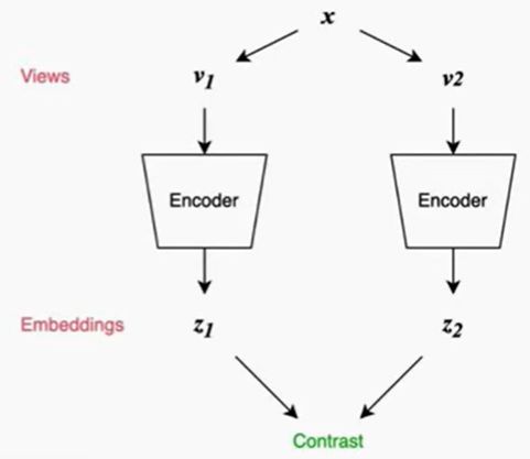
Many contrastive self-supervised learning methods use a pair of neural networks and learned from their difference
– this idea can be tracked back to Siamese Networks

• Self-organizing neural networks
  • where two neural networks take seperate but related parts of the input, and learns to maximize the agreement between the two outputs
• Siamese Networks

  • if you believe that one network F can well encode x and get a good representation f(x)

  • then, 对于两个不同的输入x1和x2，their distance can be d(x1,x2) = L(f(x1),f(x2))

  • the idea of running two identical CNN on two different inputs and then comparing them —— a Siamese network

  • Train by:

    ✅ If xi and xj are the same person, $||f(xi)-f(xj)$ is small

    ✅ If xi and xj are the different person, $||f(xi)-f(xj)$ is large

Multiple Instance Learning & Metric Learning

Predecessors of the predetestors of the recent contrastive learning techniques : multiple instance learning and metric learning

• deviate frome the typical framework of empirical risk minimization

  • define the objective function in terms of multiple samples from the dataset $\Rightarrow$ multiple instance learning

• ealy work:

  • around non-linear dimensionality reduction
  • 如multi-dimensional scaling and locally linear embedding
  • better than PCA: can preserving the local structure of data samples

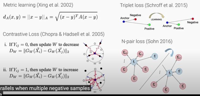
• metric learning:

  • x and y: two samples
  • A: A learnable positive semi-definite matrix

• contrastive Loss:

  • use a spring system to decrease the distance between the same types of inputs, and increase between different type of inputs

• Triplet loss

  • another way to obtain a learned metric
  • defined using 3 data points
  • anchor, positive and negative
  • the anchor point is learned to become similar to the positive, and dissimilar to the negative

• N-pair loss:

  • generalized triplet loss
  • recent 对比学习 就以 N-pair loss 为原型

Methods

• self-prediction
• Contrastive learning

Methods for Framing Self-Supervised Learning Tasks

• Self-prediction: Given an individual data sample, the task is to predict one part of the sample given the other part
  • 即 “Intra-sample” prediction

The part to be predicted pretends to be missing

• Contrastive learning: Given multiple data samples, the task is to predict the relationship among them

  • relationship: can be based on inner logics within data

    ✅ such as different camera views of the same scene

    ✅ or create multiple augmented version of the same sample

The multiple samples can be selected from the dataset based on some known logics (e.g., the order of words / sentences), or fabricated by altering the original version
即 we know the true relationship between samples but pretend to not know it

Self-Prediction

• Self-prediction construct prediction tasks within every individual data sample

  • to predict a part of the data from the rest while pretending we don’t know that part

  • The following figure: demonstrate how flexible and diverse the options we have for constructing self-prediction learning tasks

    ✅ can mask any dimensions

    

• 分类：

  • Autoregressive generation
  • Masked generation
  • Innate relationship prediction
  • Hybrid self-prediction

Self-prediction: Autoregressive Generation

• The autoregressive model predicts future behavior based on past behavior

  • Any data that comes with an innate sequential order can be modeled with regression

• Examples :

  • Audio (WaveNet, WaveRNN)
  • Autoregressive language modeling (GPT, XLNet)
  • Images in raster scan (PixelCNN, PixelRNN, iGPT)

Self-Prediction: Masked Generation

• mask a random portion of information and pretend it is missiing, irrespective of the natural sequence

  • The model learns to predict the missing portion given other unmasked information

• e.g.,

  • predicting random words based on other words in the same context around it

• Examples :

  • Masked language modeling (BERT)
  • Images with masked patch (denoising autoencoder, context autoencoder, colorization)

Self-Prediction: Innate Relationship Prediction

• Some transformation (e.g., segmentation, rotation) of one data samples should maintain the original information of follow the desired innate logic

• Examples

  • Order of image patches

    ✅ e.g., shuffle the patches

    ✅ e.g., relative position, jigsaw puzzle

  • Image rotation

  • Counting features across patches

Self-Prediction: Hybrid Self-Prediction Models

Hybrid Self-Prediction Models: Combines different type of generation modeling

• VQ-VAE + AR
  • Jukebox (Dhariwal et al. 2020), DALL-E (Ramesh et al. 2021)
• VQ-VAE + AR + Adversial

  • VQGAN (Esser & Rombach et al. 2021)

  • VQ-VAE: to learn a discrete code book of context rich visual parts

  • A transformer model: trained to auto-aggressively modeling the color combination of this code book

    

Contrastive Learning

• Goal:

  • To learn such an embedding space in which similar sample pairs stay close to each other while dissimilar ones are far apart

    

• 对比学习 can be applied to both supervised and unsupervised settings

  • when working with unsupervised data, 对比学习 is one of the most powerful approach in the self-supervised learning

• Category

  • Inter-sample classification

    the most dominant approach

    ✅ “inter-smaple”: emphasize or distinguish it from “intra-sample”

  • Feature clustering

  • Multiview coding

Contrastive Learning: Inter-Sample Classification

• Given both similar (“positive”) and dissimilar (“negative”) candidates, to identify which ones are similar to the anchor data point is a classification task

  • anchor: the original input

• How to construct a set of data point candidates:

  • The original input and its distorted version
  • Data that captures the same target from different views

• Common loss functions :

  • Contrastive loss, 2005
  • Triplet loss, 2015
  • Lifted structured loss, 2015
  • Multi-class n-pair loss, 2016
  • Noise contrastive estimation, 2010
  • InfoNCE, 2018
  • Soft-nearest neighbors loss, 2007, 2019

Loss function 1: Contrastive loss

• 2005

• Works with labelled dataset

• Encoder data into an embedding vector

  • such that examples from the same class have similar embeddings and samples from different classes have different ones

• Given two labeled data pairs $(x_i,y_i)$ and $(x_j,y_j)$:

  

Loss function 2: Triplet loss

• Triplet loss (Schroff et al. 2015)

  • learns to minimize the distance between the anchor $x$ and positive $x+$ and
  • maximize the distance between the anchor $x$ and negative $x-$ at the same time

• Given a triplet input $(x,x^{+},x^{-})$

  

Triplet (三胞胎) loss: because it demands an input triplet containing one anchor, one positive and one negative

Loss function 3: N-pair loss

• N-Pair loss (Sohn 2016)
  • generalizes triplet loss to include comparison with multiple negative samples
• Given oen positive and N-1 negative samples:
  • $\{x,x^{+},x_1^{-},...,x_{N-1}^{-}\}$

Loss function 4: Lifted structured loss

• Lifted structured loss (Song et al. 2015):

  • utilizes all the pairwise edges within one training batch for better computational efficiency

    

• 对于大规模训练，batchsize经常非常大

  • means we have many samples within one batch
  • can construct multiple similar or dissimilar pairs
  • Lifted structured loss: utilize all the paragraphs edges of relationship within one training batch
  • improve compute efficiency as it incorporates more information within one batch

Loss function 5: Noise Contrastive Estimation (NCE)

• Noise contrastive Estimation (NCE): Gutmann & Hyvarinen 2010

  • runs logistic regression to tell apart the target data from noise

• Given target sample distribution p and noise distribution q:

  

• initially proposed to learn word embedding in 2010

Loss function 6: InfoNCE

• InfoNCE (2018)

  • Uses categorical cross-entropy loss to identify the positive sample amongst a set of unrelated noise samples

• Given a context vector c, the positive sample should be drawn from the conditional distribution $(p(x|c))$

  • while N-1 negative samples are drawn from the proposal distribution p(x), independent from the context c

• The probability of detecting the positive sample correctly is:

  

Loss function 7: Soft-Nearest Neighbors Loss

• Soft-Nearest Neighbors Loss (Frosst et al. 2019): extends the loss function to include multiple positive samples given known labels
• Given a batch of samples $\{x_i,y_i\}{|}_{i=1}^B$

  • known labels may come from supervised dataset or fabricated with data augmentation

  • temperature term: tuning how concentrated the feature space

    

Contrastive Learning: Feature Clustering

• Find similar data samples by clustering them with learned features

• core idea : Use clustering algorithms to assign pseudo lables to samples such that we can run intra-sample contrastive learning

• Examples:

  • Deep Cluster (Caron et al 2018)

  • Inter CLR (Xie et al 2021)

    

Contrastive Learning: Multiview Coding

• Apply the InfoNCE objective to two or more different views of input data

  

• Became a mainstream contrastive learning method

  • AMDIM (Bachman et al 2019)
  • Contrastive multiview coding (CMC, Tian et al 2019) 等

Contrastive Learning between Modalities

• Views can be from paired inputs from two or more modalities

  • CLIP (Radford et al 2021)、ALIGN (Jia et al 2021)：enables zero-shot classification, cross-modal retrieval, guided image generation

  • CodeSearchNet (Husain et al 2019): contrast learning between text and code

    

Pretext tasks

Recap: Pretext Tasks

• Step 1: Pre-train a model for a pretext task

• Step 2: Transfer to applications

  

Pretext Tasks: Taxonomy

• Generative
  • VAE
  • GAN
  • Autoregressive
  • Flow-based
  • Diffusion
• Self-Prediction
  • Masked Prediction (Denoising AE, Context AE)
  • Channel Shuffling (colorization, split-brain)
• Innate Relationship
  • Patch Positioning
  • Image Rotation
  • Feature Counting
  • Contrastive Predictive Coding
• Contrastive

  • Instance Discrim

  • Augmented Views

  • Clustering-based

    

Image / Vision Pretext Tasks

Image Pretext Tasks: Varizational AutoEncoders

• Auto-Encoding Variational Bayes (Kingma et al. 2014)

  

• Image generation：

  • itself is an immensely broad field that deserves an entire tutorial or more
  • but can also serve as representation learning

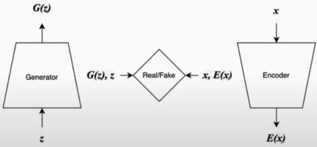
Image Pretext Tasks: Generative Adversial Networks

• Jointly train an encoder, additional to the usual GAN

  • Bidirectional GAN

  • Adversarially Learned Inference

    

• GAN Inversion: learning encoder post-hoc and/or optimizing for given image

Vision Pretext Tasks: Autoregressive Image Generation

• Neural autoregressive density estimation (NADE)
• Pixel RNN, Pixel CNN
  • Use RNN and CNN to predict values conditioned on the neighboring pixels
• Image GPT
  • Uses a transformer on discretized pixels and was able to obtain better representation than building of supervised approaches

Vision Pretext Tasks: Diffusion Model

• Diffusion Modeling :

  • Follows a Markov chain of diffusion steps to slowly add random noise to data

  • and then learn to reverse the diffusion process to construct desired data samples from the noise

    

Vision Pretext Tasks: Masked Prediction

• Denoising autoencoder (Vincent et al. 2008)

  • Add noise = Randomly mask some pixels

  • Only reconstruction loss

    

• Context autoencoder (Pathak et al 2016)

  • Mask a random region in the image

  • Reconstruction loss + adversial loss

  • adversial loss: tries to make it difficult to distingusih between the painting produced by the model and the actual image

    

Vision Pretext Tasks: Colorization and More

can not only be on the pixel value itself, but also on any subset of information from the image

• Image Colorization

  • Predict the binned CIE Lab color space given a grayscale image

• Split-brain autoencoder

  • Predict a subset of color channels from the rest of channels
  • Channels: luminosit, color, depth, etc.

  

In order to get representation that transfer well to downstream tasks

Vision Pretext Tasks: Innate Relationship Prediction

• Learn the relationship among image patches:
  • Predict relative positions between patches
  • Jigsaw Puzzle using patches

• RotNet: predict which rotation is applied (Gidaris et al. 2018)
  • Rotation does not alter the semantic content of an image
• Representation Learning by Learning to Count (Noroozi et al. 2017)
  • Counting features across patches without labels, using equivariance of counts
  • ie, learns a function that counts visual primitives in images

Contrastive Predictive Coding and InfoNCE

• Contrastive Predictive Coding (CPC) (van den Oord et al 2018)
  • Classify the “future” representation amongst a set of unrelated “negative” samples
  • an autoregressive context predictor is used to classify the correct future patches

• minimizing the loss function 等价于 maxmizing a lower bound to the mutual information between the predicted context $c_t$ and the future patch $x_{t+k}$
  • 相当于预测的数据的latent representation最准确

CPC has been highly influential in contrastive learning

• showing the effectiveness of causing the problem as an entire sample classification task

Vision Pretext Tasks: Inter-Sample Classification

• Example CNN
• Instance-level discrimination

  • Each istance is a distinct calss of its own

    # classes = # training samples

  • Non-parametric softmax that compares features

  • Memory bank for stroing representations of past samples $V=V\{i\}$

The model learns to scatter the feature vectors in the hypersphere while mapping visually similar images into closer regions

Vision Pretext Tasks: Contrastive Learning

• Common approach:
  • Positive: make multiple views to one images and consider the image and its distorted version as similar pairs
  • Negative: different images are treated dissimilar

一个自然的问题：Is there better ways to creat multiview images? $\downarrow$

Vision Pretext Tasks: Data Augmentation and Multiple Views

• Augment Multiscale Deep InfoMax
  • AMDIM, Bachman 2019
  • Views from different augmentations
  • create multiple views from one input image
• Contrastive Multiview Coding
  • CMC
  • Multiple views from different channels or semantic segmentation labels of the image as different views from a single image
• Pretext-Invariant Representation Learning
  • Jigsam transformation
  • (as an input transform)

Vision Pretext Tasks: Inter-Sample Classification

MoCo

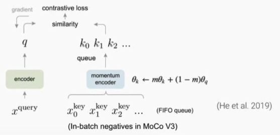
• MoCo (Momentum Contrast; He et al. 2019)

  • Memory bank is a FIFO queue now
  • The target features are encoded using a momentum encoder $\Rightarrow$ 一个batch付出很小的代价即可获得更多的negative samples
  • shuffling BN: 缓解BN对self-supervised learning的不利影响
    - MOCO v2:
  • MLP projection head
  • stronger data augmentation （添加了模糊）
  • Cosine learning rate schedule

  

• MoCo v3:

  • Use Vision Transformer to replace ResNet
  • in-batch negatives

  

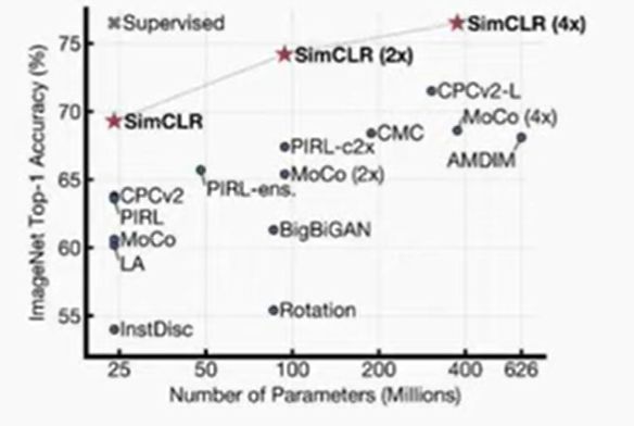
SimCLR

• SimCLR (Simple framework for Contrastive Learning of visual Representation)

  • Contrastive learning loss

  • f() – base encoder

  • g() – projection head layer

  • In-batch negative samples

    ✅ Use large batches to have sufficient number of negative inputs

fully symmetric;

• SimCLR v2
  • Larger ResNet models
  • Deeper g()
  • Memory bank

Barlow Twins

• Barlow Twins (Zbontar et al. 2021)

  • Learn to make the cross-correlation matrix between two output features for two distorted version of the same sample close to the identity
  • Make it as diagonal as possible
  • because: if the individual features are efficiently encoded, they shouldn’t be encoding information that is redundant between any pairs $\Rightarrow$ their corrleation should be zero

  

Vision Pretext Tasks: Non-Contrastive Siamese Networks

Learn similarity representations for different augmented views of the same sample, but no contrastive component involving negative samples

• the objective is just minimizing the L2 distance between features encoded from the same image

• Bootstrap Your Own Latent (BYOL, et al. )

  • Momentum-encoded features as the target

• Simsiam (Chen 2020)

  • No momentum encoder
  • Large batch size unnecessary

• BatchNorm seems to be playing an important role

  • might implicityly providing contrastive learning signal

Vision Pretext Tasks: Feature Clustering with K-Means

another major technology for self-supervised learning:

• to learn from clusters of features

• DeepCluster (Caron et al. 2018)
  • Iteratively clusters features via k-means
  • then, uses cluster assignments as pseudo lables to provide supervised signals
• Online DeepCluster (Zhan et al. 2020)
  • Performs clustering and netwrok update simultaneously rather than alternatingly

• Prototypical Cluster Learning (PCL, Li et al. 2020)
  • Online EM for clustering
  • combined with InfoNCE for smoothness

Vision Pretext Tasks: Feature Clustering with Sinkhorm-Knopp

Sinkhorm-Knopp: a cluster algorithm based on OT

• SeLa (Self-Labelling, Asano et al. 2020)
• SwAV (Swapping Assignments between multiple Views; Caron et al. 2020)
  • Implicit clustering via a learned prototype code (“anchor clusters”)
  • Predict cluster assignment in the other column

Vision Pretext Tasks: Feature Clustering to improve SSL

In this approach, nobel ideas based on clustering are designed to be used in conjunction with other SSL methods

• InterCLR (Xie et al. 2020)
  • Inter-sample contrastive pairs are constructed according to pseudo labels obtained by clustering
  • 即让对比学习的正样本也可以来自不同的图片 (而不是只能通过Multi-view) using pseudolabels from an online k-means clustering
• Divide and Contraset (Tian et al. 2021)

  • Train expert models on the clustered datasets and then distill the experts into a single model

  • to improve the performance of other self-supervised learning models

    

Vision Pretext Tasks: Nearest-Neighbor

• NNCLR (Dwibedi et al. 2021)

  • Contrast with the nearest neighbors in the embedding space

    ✅ to serve as the positive and negtive in contrastive learning

  • Allows for lighter data augmentation for views

    

Vision Pretext Tasks: Combining with Supervised Loss

• Combine supervised loss + self-supervised learning
  • Self-supervised semi-supervised learning (S4L, Zhai et al 2019)
  • Unsupervised data augmentation (UDA, Xie et al 2019)
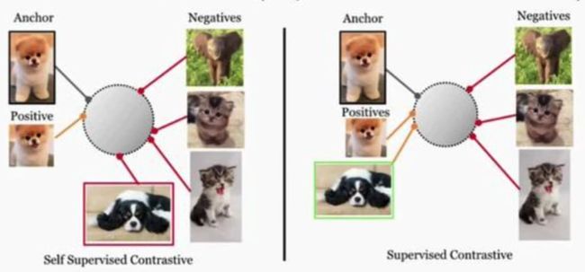
• Use known labels for contrastive learning

  • Supervised Contrastive Loss (SupCon; Khosla et al. 2021)

    ✅ less sensitive to hyperparameter choices

Video Pretext Tasks

Video Pretext Tasks: Innate Relationship Prediction

• Most image pretext tasks can be applied to videos
• However, with an additional time dimension, much more information about the video shot configuration or the physical world can be extracted from videos
  • Predicting object movements
  • 3D motion of camera

Video Pretext Tasks: Optical Flow

Tracking object movement tracking in time

• Tracking movement of image patches (Wang & Gupta, 2016)

• Segmentation based on motion (Pathak et al. 2017)

Video Pretext Tasks: Sequence Ordering

• Temporal order Verification

  • Misra et al. 2016

  • Fernando et al. 2017

  • 判断顺序是否正确

    

• Predict the arrow of time, forward or backward

  • Wei et al. 2018
  • classify whether the sequene is moving forward or backward in time
  • outperform the temporal order verification model

Video Pretext Tasks: COlorization

• Tracking emerges by colorizing videos (Vondrick et al. 2018)

  • Copy colors from a reference frame to another target frame in grayscale

  • by leverage the natural temporal coherence of colors across video frames

    

• Tracking emerges by colorizing videos (Vondrick et al. 2018)

  • Used for video segmentation or human pose estimation without fine-tuning

    ✅ because the model can move the colored markings in the labeled input image directly in the prediction

Video Pretext Tasks: Contrastive Multi-View Learning

• TCN (Sermanet et al. 2017)

  • Use triplet loss

  • Different viewpoints at the same timestep of the same scene should share the same embedding, while embedding should vary in time, even of the same camera viewpoint

    

• Multi-frame TCN (Dwibedi et al. 2019)

  • Use n-pairs loss
  • Multiple frames are aggregated into the embedding

Video Pretext Task: Autoregressive Generation

Because video files are huge, generating coherent continuous of video has been a difficult task

• Predicting videos with VQ-VAE (Walker et al. 2021)

  • first: learning to discretized the video into latent codes using VQ-VAE

  • then: learning to auto regressively generate the frames using pixel cnn or transformers

  • Combining VQ-VAE and autogressively models to generate high dimensional data $\Rightarrow$ is a very powerful generating model

    

• VideoGPT: Video generation using VQ-VAE and Transformers (Yan et al. 2021)

• Jukebox (Dhariwal et al. 2020)

  • learning 3 different level of VQ-VAE using 3 different compression ratio
  • resulting 3 sequence of discrete code
  • then use them to generate new music

• CALM (Castellon et al. 2021)
  • Jukebox representation for MIR tasks
• TagBox (Manilow et al. 2021)

  • Source separation by steering Jukebox’ latent space

    

Audio Pretext Tasks

Audio Pretext Tasks: Contrastive Learning

• COLA (Saeed et al. 2021)
  • Assigns high similarity between audio clip extracted from the same recording and low similarity to clips from different recordings
  • predicts a pari of encoded features are from the same recording or not
• Multi-Format audio contrastive learning

  • assigns high similarity between the raw audio format and the corresponding spectral representation

  • maximizing agreement between between features included from the raw waveform and he spectrogram formats

    

Audio Pretext Task: Masked Languagee Modeling for ASR

ASR: Automatic speech recognition

• Wav2Vec 2.0 (Baevski et al. 2020)

  • applies contrast siblings on the representation of mask portion of the audio

    ✅ to learn discrete tokens from them

  • speech recognition models: trained on these token, show better performance compared to those trained on conventional audio features / raw audio

• HuBERT (Hsu et al. 2021, FAIR)

  • learned by alternating between an offline cadence clustering step and optimizing for cluster assignment prediction (similar to deep cluster)

• Also employed by SpeechStew (Chan et al. 2021), Big SSL (Zhang et al. 2021)

  

Multimodal Pretext Tasks

applied to multimodal data, although the difinition of self-supervised learning gets kind of blurry here depending on whether you consider a multi-modal dataset as single unlabeled dataset or as if one modality gives supervision to another modality

• MIL-NCE (Miech et al. 2020)

  • Find matching narration with video

  • trained constrastively to find matching narration with video, which can not only use for correcting misalignment in videos but also for action recognition, text to video retrieval, action localization and action segmentation

    

• CLIP (Radford et al. ), ALIGN (Jia et al. 2021)

  • Contrast text and image embeddings from paired data

Language Pretext Tasks

Language Pretext Tasks: Generative Language Modeling

• Pretrained language models:

  • They all rely on unsupervised text and try to predict one sentence from the context
  • only depend on the natural order of words and sequences

• Some examples: changed the landscape of NLP research quite a lot

  • GPT

    ✅ Autogressive;

    ✅ predict the next token based on the previous tokens

  • BERT

    ✅ as a bi-directional transformer model

    ✅ Masked language modeling (MLM)

    ✅ Next sentence prediction (NSP) $\Rightarrow$ a binary classifier for telling whether one sentence is the next sentence of the other

  • ALBERT

    ✅ Sentence order prediction (SOP) $\Rightarrow$ Positive sample: a pair of two consecutive segments from the same document; Negative sample: same as above but with the segment order switch

  • ELECTRA

    ✅ Replaced token detection (RTD) $\Rightarrow$ random tokens are replaced and considered corrected, in parallel a binary discriminator is trained together with the generative model to predict whether each token has been replaced

Language Pretext Tasks: Sentence Embedding

• Skip-thought vectors (Kiros et al. 2015)

  • Predict sentences based on other sentences around

• Quick-thought vectors (Logeswaran & Lee, 2018)

  • Identify the correct context sentence among other contrastive sentences

  

• IS-BERT (“Info-Sentence BERT”; Zhang et al. 2020)

  • matual information maximization

• SimCSE (“Simple Contrastive learning of Sentence Embeddings”; Gao et al. 2021)

  • Predict a sentence from itself with only dropout noise
  • One sentence gets two different versions of dropout augmentations

  

• Most of the models for learning sentence embedding relies on supervised NLI (Natural Language Inference) datasets, such as SBERT (Reimers & Gurevych 2019), BERT-flow
• Unsupervised sentence embedding models (e.g., unsupervised SimCSE) still have performance gap with the supervised version (e.g., supervised SimCSE)

Training Techniques

• Data augmentation
• In-batch negatives samples
• Hard negative mining
• Memory bank
• Large batchsize

contrastive learning can provide good results in terms of transfer performance

Techniques: Data augmentation

• Data augmentation setup is critical for learning good embedding

  • and generalizable embdding features

• 方法：

  • Introduces the non-essential variations into examples without modifying semantic meanings
  • $\Rightarrow$ thus encourages the model to learn the essential part within the representation

image augmentation; text augmentation

Techniques: Data augmentation – Image Augmentation

• Basic Image Augmentation:

  • Random crop
  • color distortion
  • Gaussian blur
  • color jittering
  • random flip / rotation
  • etc.

• Augmentation Strategies

  • AutoAugment (Cubuk, et al. 2018): Inspired by NAS
  • RandAugment (Cubuk et al. 2019): reduces NAS search space in AutoAugment
  • PBA (Population based augmentation; Ho et al. 2019): evolutionary algorithms
  • UDA (Unsupervised Data Augmentation ,Xie et al. 2019): select augmentation strategy to minimize the KL divergencec between the predicted distribution over an unlabelled example and its unlabelled augmented version

• Image mixture

  • Mixup (Zhang et al. 2018): weighted pixel-wise combination of two images

    ✅ to create new sampls based on existed ones

  • Cutmix (Yun et al 2019): mix in a local region of one image into the other

  • MoCHi (Mixing of Contrastive Hard Negatives): mixture of hard negative samples

    ✅ explicitly maintains a queue of some number of negative samples sorted by similarity to the query in descending order $\Rightarrow$ the first couple samples in the queue should be the hardest and negative samples $\Rightarrow$ then new hard negative can be created by mixing images in this queue together or even with the query

Techniques: Data augmentation – Text Augmentation

• Lexical (词汇的) Edits.

  • (Just changing the words or tokens)

  • EDA (Easy Data Augmentation; Wei & Zhou 2019): Synonym replacement, random insertion / swap / deletion

  • Contextual Augmentation (Kobayashi 2018): word substition by BERT prediction

    ✅ try to find the replacement words using a bi-directional language model

• Back-translation (Sennrich et al. 2015)

  • augments by first translating it to another language and then translating it back to the original language

    ✅ depends on the translation model $\Rightarrow$ the meaning should stay largely unchanged

  • CERT (Fang et al. 2020) generates augmented sentences via back-translation

• Dropout and Cutoff

  • SimCSE uses dropout (Gao et al. 2021)

    ✅ drouput: a universal way to apply transformnation on any input

    ✅ SimCSE: use drouput to creat different copies of the same text $\Rightarrow$ universial because it doe not need expert knowledege about the attributes of this input modality (it is changes on the architecture level)

  • Cutoff augmentation for text (Shen et al. 2020)

    ✅ masking random selected tokens, feature columns, spans

  

Hard Negative Mining

What is “hard negative mining”

• Hard negative samples are different to learn
  • They should have different labels from the anchor samples
  • But the embedding features may be very close
• Hard negative mining is important for contrastive learning
• Challenging negative samples encourages the model to learn better representations that can distinguish hard negatives from true positives

Explicit hard negative mining

• Extract task-specific hard negative samples from labelled datasets
  • e.g., “contradiction” sentence pairs from NLI datasets.
  • (Most sentence embedding papers)
• Keyword based retrieval
  • can be found by classic information retrieval models (Such as BM25)
• Upweight the negative sample probability to be proportional to its similarity to the anchor sample
• MoCHi: mine hard negative by sorting them according to similarity to the query in descending order

Implicit hard negative mining

• In-batch negative samples
• Memory bank (Wu et al. 2018, He et al. 2019)
  • Increase batch size
• Large batch size via various training parallelism

Need large batchsize

Theories

Why does contrastive learning work?

Contrastive learning captures shared information betweem views

• InfoNCE (van den Oord et al. 2018)

  • is a lower bound to MI (Mutual information) between views:

  

• Minimizing InfoNCE leads to maximizing the MI between view1 and view2

  • 因此，minimizing the inforNCE loss $\Rightarrow$ the encoder are optimizing the embedding space to retain as much information as possible that exsited between the two views
  • The info max principle in contrastive learning

  

• Q: How can we design good views?

  • augmentations are crucial for the performance

The InfoMin Principle

• Optimal views are at the sweet spot where it only encodes useful informnation for transfer

  • Minimal sufficient encoder depends on downstream tasks (Tian et al. 2020)

  • Composite loss for finding the sweet spot (Tsai et al. 2020)

    ✅ helps converging to a minimal sufficient encoder

To perform well in transfer learning $\Rightarrow$ we want our model to capture the mutual information between the data x and the downstream label y $I(x;y)$

• if the mutual information between the views ($I(v_1;v_2)$) is smaller than $I(x;y)$ $\Rightarrow$ the model would fail to capture useful information for the downstream tasks
• Meanwhile, if the mutual information between the views are too large $\Rightarrow$ would have excess information that is unrelated to the downstream tasks $\Rightarrow$ the transfor performance would decrease due to the noise
• $\Rightarrow$ there is a sweet spot $\Rightarrow$ the minimal sufficient encoder

• This shows:
  • The optimal views are dependent on the downstream tasks

Alignment and Uniformity on the Hypersphere

• Contrastively learned features are more uniform and aligned

  • Uniform : features should be distributed uniformly on the hypershere $S^d$
  • Aligned : features from two views of the same input should be the same

  

• compared with random initialized network or a network trained with the supervised learning
• also measured the alignment measuring how close the distance between features from two views of the same input is

Dimensional Collapse

• Contrastive methods sometimes suffer from dimensional collapse (Hua et al. 2021)
  • Features span lower-dimensional subspace instead
  • (Learned features span lower dimensional subspace instead of using the full dimensionality)
• Two causes demonstrated by Jing et al (2021)
  • 1 Strong augmentation while creating the views
  • 2 implicit regularization caused by the gradient decent dynamics

Provable Guarantees for Contrastive Learning

• Sampling complexity decreases when:
  • Adopting contrastive learning objectives (Arora et al. 2019)
  • Predicting the known distribution in teh data (Lee et al. 2020)
• Linear classifier on learned representation is nearly optimal (Tosh et al. 2021)
• Spectral Contrastive Learning (HaoChen et al. 2021)
  • based on a spectral decomposition of the augmentation graph

总之，对比学习理论起到了很大作用，但仍有很长的路要走

Feature directions

briefly discuss a few open research questions and areas of work to look into

Future Directions

• Large batch size $\Rightarrow$ improved transfer performance

• High-quality large data corpus $\Rightarrow$ better performance

  • Learning from synthetic or Web data
  • Measuring dataset quality and filtering / active learning $\Rightarrow$ better control over data quality

• Efficient negative sample selection

  • to do hard negative mining
  • (lage batchsize is not enough because batchsize cannot go to infinity)

• Combine multiple pretext tasks

  • How to combine
  • Best strategies

  

• Data augmentation tricks have critical impacts but are still quite ad-hoc

  • Modality-dependent: 大多数增强方法仅适用于单个modality $\Rightarrow$ most of them are handcrafted by human

  • Theoretical foundations

    ✅ e.g., on why certain augmentation works better than others

    ✅ to guide us to find more efficient data augmentation

• Improving training efficiency

  • Self-supervised learning methods are pushing the deep learning arms race (军备竞赛)

    ❌ increase of model size and training batch size

    ❌ $\Rightarrow$ leads to increase the cost both economically and environmentally

  • Direct impacts on the economical and environmental costs

• Social biases in the embedding space

  • Early work in debiasing word embedding
  • Biases in Dataset