尚硅谷-机器学习与深度学习笔记

本文章仅仅记录本人的学习过程，侵权删。
视频地址：https://www.bilibili.com/video/BV1zb411P7iV
代码和数据：代码和数据

P3. 人工智能的发展和现状

什么是人工智能：

人工智能（Artificial Intelligence） ，英文缩写：AI 。它是研究，开发用于模拟、延伸和扩展人的智能的理论、方法、技术及应用系统的一门新的技术科学。人工智能是计算机科学的一个分支，它试图了解智能的实质，并生产出一种新的能以人类智能相识的方式作出反应的智能机器。

应用场景：

• 机器人
• 语音识别
• 图像识别
• 自然语言处理
• 专家系统
• 知识工程
• 机器学习

人工智能是对人的意识，思维的信息过程的模拟。人工智能不是人的智能，但能像人那样的思考，甚至超过人的智能。

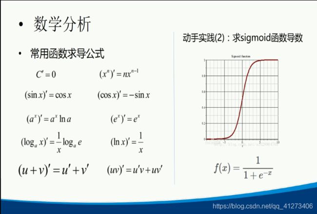
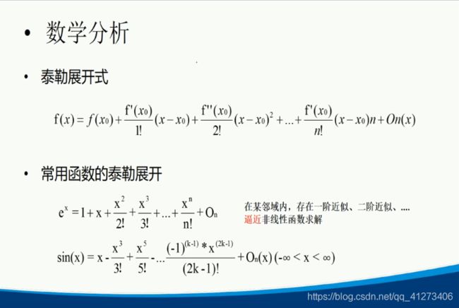
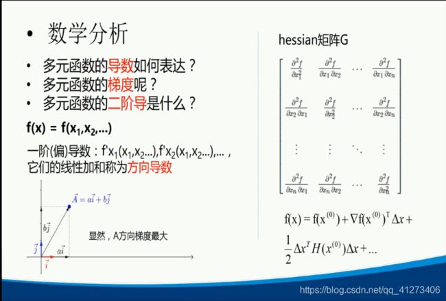
P4.数学分析基础

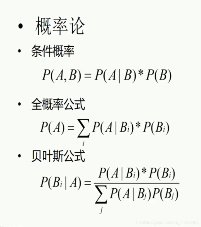
P5. 线性代数与概率论基础

P6.机器学习基本概念

从学习的方式上分为：

• 监督学习
• 无监督学习
• 半监督学习
• 强化学习

从学习结果上分为：

• 回归
• 分类

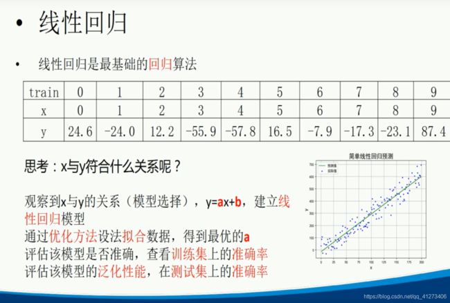
P7.线性回归模型

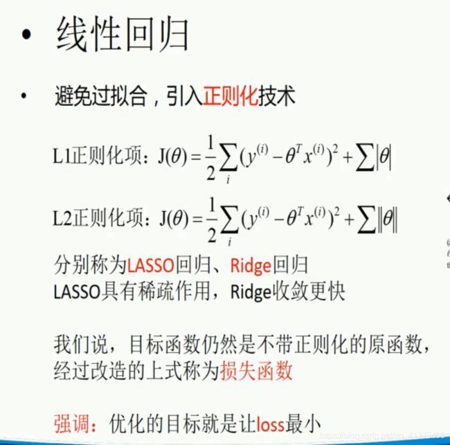
P8.线性回归习题与总结

import numpy as np
import pandas as pd
import matplotlib as mpl
import matplotlib.pyplot as plt

from sklearn.model_selection import train_test_split
from sklearn.linear_model import LinearRegression
from sklearn.linear_model import Lasso
from sklearn.linear_model import Ridge
from sklearn.linear_model import ElasticNet

from sklearn.preprocessing import PolynomialFeatures, StandardScaler
from sklearn.pipeline import Pipeline


def generate_lr_train_data(polynomial = False):
    if not polynomial:
        f = open("./simple_lr.data", "w")
        for i in range(200):
            f.write("%s %s\n" % (i, i * 3 + np.random.normal(0, 50)))
    else:
        f = open("./polynomial_lr.data", "w")
        for i in range(200):
            f.write("%s %s\n" % (i, 1 / 20 * i * i + i + np.random.normal(0, 80)))
    f.close()


def read_lr_train_data(polynomial = False):
    if not polynomial:
        return pd.read_csv("./simple_lr.data", header = None)
    else:
        return pd.read_csv("./polynomial_lr.data", header = None)


def simple_linear_regression():
    # if polynomial used
    polynomial = True

    # generate simple lr train data
    generate_lr_train_data(polynomial)

    # read simple lr train data 读取数据
    lr_data = read_lr_train_data(polynomial)
    clean_data = np.empty((len(lr_data), 2))
    for i, d in enumerate(lr_data.values):#数据清洗，去除重复行
        clean_data[i] = list(map(float, list(d[0].split(' '))))

    x, y = np.split(clean_data, (1, ), axis = 1) # split array to shape [:1],[1:] 切割
    y = y.ravel()
    print("样本个数：%d，特征个数：%d" % x.shape)

	#划分训练集和测试集
    x_train, x_test, y_train, y_test = train_test_split(x, y, train_size = 0.7, random_state = 0)
    model = Pipeline([("ss", StandardScaler()),
        ("polynomial", PolynomialFeatures(degree = 60, include_bias = True)),#升幂
       	#("linear", Lasso(alpha=10))
        ("linear", LinearRegression())  # 这里可以在选择普通线性回归、Lasso/Ridge
    ])

    print("开始建模")
    model.fit(x_train, y_train)
    y_pred = model.predict(x_train)
    print("建模完毕")

    # 绘制前调整数据
    order = x_train.argsort(axis=0).ravel()
    x_train = x_train[order]
    y_train = y_train[order]
    y_pred = y_pred[order]

    # 绘制拟合曲线
    mpl.rcParams["font.sans-serif"] = ["simHei"]
    mpl.rcParams["axes.unicode_minus"] = False
    plt.figure(facecolor = "w", dpi = 200)
    plt.scatter(x_train, y_train, s = 5, c = "b", label = "实际值")
    plt.plot(x_train, y_pred, "g-", lw = 1, label = "预测值")
    plt.legend(loc="best")
    plt.title("简单线性回归预测", fontsize=18)
    plt.xlabel("x", fontsize=15)
    plt.ylabel("y", fontsize=15)
    plt.grid()
    plt.show()


if __name__ == "__main__":
    simple_linear_regression()

用(“linear”, Lasso(alpha=10))产生的：

用(“linear”, LinearRegression())产生的：

P9.Logistic回归模型与练习

import numpy as np
import pandas as pd

from sklearn.linear_model import LogisticRegression
from sklearn.preprocessing import StandardScaler, PolynomialFeatures
from sklearn.pipeline import Pipeline

import matplotlib as mpl
import matplotlib.pyplot as plt


if __name__ == "__main__":
    path = 'iris.data'
    data = pd.read_csv(path, header=None)
    data[4] = pd.Categorical(data[4]).codes # one-hot 类似特征矩阵 有就是1，没有就是0

    print(data[4].unique())
    x, y = np.split(data.values, (4,), axis=1)

    x = x[:, :2]
    lr = Pipeline([('sc', StandardScaler()), ('poly', PolynomialFeatures(degree=2)), ('clf', LogisticRegression())])

    lr.fit(x, y.ravel())
    y_hat = lr.predict(x)
    y_hat_prob = lr.predict_proba(x)
    np.set_printoptions(suppress=True)

    print('y_hat = \n', y_hat)
    print('y_hat_prob = \n', y_hat_prob)
    print('准确率：%.2f%%' % (100 * np.mean(y_hat == y.ravel())))

    # 画图
    N, M = 500, 500  # 横纵各采样多少个值
    x1_min, x1_max = x[:, 0].min(), x[:, 0].max()  # 第0列的范围
    x2_min, x2_max = x[:, 1].min(), x[:, 1].max()  # 第1列的范围
    t1 = np.linspace(x1_min, x1_max, N)
    t2 = np.linspace(x2_min, x2_max, M)
    x1, x2 = np.meshgrid(t1, t2)  # 生成网格采样点
    x_test = np.stack((x1.flat, x2.flat), axis=1)  # 测试点

    mpl.rcParams['font.sans-serif'] = ['simHei']
    mpl.rcParams['axes.unicode_minus'] = False

    y_hat = lr.predict(x_test)  # 预测值
    y_hat = y_hat.reshape(x1.shape)  # 使之与输入的形状相同

    plt.figure(facecolor='w')
    plt.pcolormesh(x1, x2, y_hat)  # 预测值的显示
    plt.scatter(x[:, 0], x[:, 1], c=np.squeeze(y), s=50)  # 样本的显示
    plt.xlabel('花萼长度', fontsize=14)
    plt.ylabel('花萼宽度', fontsize=14)
    plt.xlim(x1_min, x1_max)
    plt.ylim(x2_min, x2_max)
    plt.grid()
    plt.title("Logistic回归-鸢尾花", fontsize=17)
    plt.show()

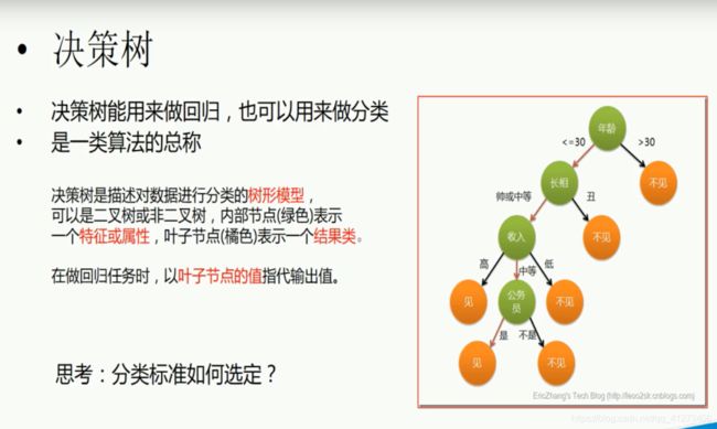
P10.决策树

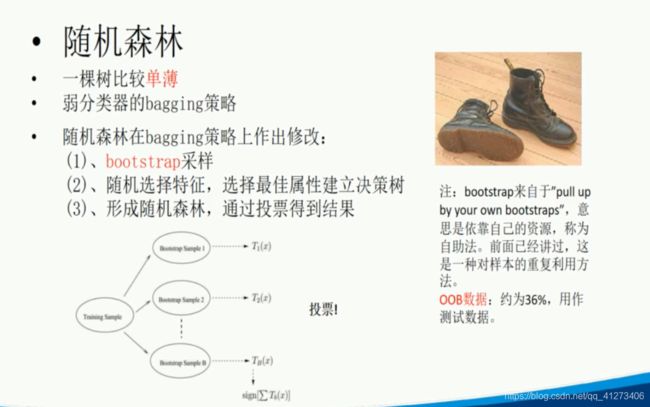
P11.随机森林

import numpy as np
import pandas as pd
import xgboost as xgb
from sklearn.model_selection import train_test_split  # cross_validation


def iris_type(s):
    it = {b'Iris-setosa': 0, b'Iris-versicolor': 1, b'Iris-virginica': 2}
    return it[s]


if __name__ == "__main__":
    path = 'iris.data'  # 数据文件路径
    data = np.loadtxt(path, dtype=float, delimiter=',', converters={4: iris_type})
    data = pd.read_csv(path, header=None)
    x, y = data[list(range(4))], data[4]
    y = pd.Categorical(y).codes
    x_train, x_test, y_train, y_test = train_test_split(x, y, random_state=1, test_size=50)

    data_train = xgb.DMatrix(x_train, label=y_train)
    data_test = xgb.DMatrix(x_test, label=y_test)
    watch_list = [(data_test, 'eval'), (data_train, 'train')]
    param = {'max_depth': 2, 'eta': 0.3, 'silent': 1, 'objective': 'multi:softmax', 'num_class': 3}

    bst = xgb.train(param, data_train, num_boost_round=6, evals=watch_list)
    y_hat = bst.predict(data_test)
    result = y_test.reshape(1, -1) == y_hat
    print('正确率:\t', float(np.sum(result)) / len(y_hat))

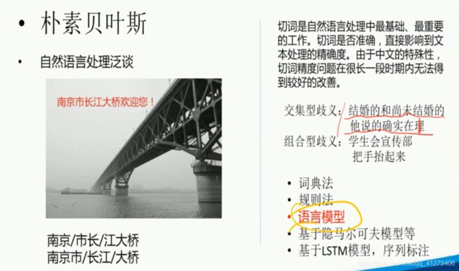
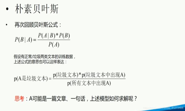
P12.朴素贝叶斯

import numpy as np

from sklearn.naive_bayes import MultinomialNB, BernoulliNB
from sklearn.datasets import fetch_20newsgroups
from sklearn.feature_extraction.text import TfidfVectorizer
from sklearn.model_selection import GridSearchCV
from sklearn import metrics

from time import time
from pprint import pprint
import matplotlib.pyplot as plt
import matplotlib as mpl


def make_test(classfier):
    print('分类器：', classfier)
    alpha_can = np.logspace(-3, 2, 10)
    model = GridSearchCV(classfier, param_grid={'alpha': alpha_can}, cv=5)
    model.set_params(param_grid={'alpha': alpha_can})

    t_start = time()
    model.fit(x_train, y_train)
    t_end = time()

    t_train = (t_end - t_start) / (5 * alpha_can.size)
    print('5折交叉验证的训练时间为：%.3f秒/(5*%d)=%.3f秒' % ((t_end - t_start), alpha_can.size, t_train))
    print('最优超参数为：', model.best_params_)

    t_start = time()
    y_hat = model.predict(x_test)
    t_end = time()
    t_test = t_end - t_start
    print('测试时间：%.3f秒' % t_test)
    acc = metrics.accuracy_score(y_test, y_hat)
    print('测试集准确率：%.2f%%' % (100 * acc))
    name = str(classfier).split('(')[0]

    index = name.find('Classifier')
    if index != -1:
        name = name[:index]
    return t_train, t_test, 1 - acc, name


if __name__ == "__main__":
    remove = ('headers', 'footers', 'quotes')
    categories = 'alt.atheism', 'talk.religion.misc', 'comp.graphics', 'sci.space' # 选择四个类别进行分类

    # 下载数据
    data_train = fetch_20newsgroups(subset='train', categories=categories, shuffle=True, random_state=0, remove=remove)
    data_test = fetch_20newsgroups(subset='test', categories=categories, shuffle=True, random_state=0, remove=remove)

    print('训练集包含的文本数目：', len(data_train.data))
    print('测试集包含的文本数目：', len(data_test.data))
    print('训练集和测试集使用的%d个类别的名称：' % len(categories))

    categories = data_train.target_names
    pprint(categories)
    y_train = data_train.target
    y_test = data_test.target
    print(' -- 前10个文本 -- ')
    for i in np.arange(10):
        print('文本%d(属于类别 - %s)：' % (i + 1, categories[y_train[i]]))
        print(data_train.data[i])
        print('\n\n')

    # tf-idf处理
    vectorizer = TfidfVectorizer(input='content', stop_words='english', max_df=0.5, sublinear_tf=True)
    x_train = vectorizer.fit_transform(data_train.data)
    x_test = vectorizer.transform(data_test.data)
    print('训练集样本个数：%d，特征个数：%d' % x_train.shape)
    print('停止词:\n', end=' ')

    #pprint(vectorizer.get_stop_words())
    feature_names = np.asarray(vectorizer.get_feature_names())

    # 比较分类器结果
    clfs = (MultinomialNB(), BernoulliNB())
    result = []
    for clf in clfs:
        r = make_test(clf)
        result.append(r)
        print('\n')

    result = np.array(result)
    time_train, time_test, err, names = result.T
    time_train = time_train.astype(np.float)
    time_test = time_test.astype(np.float)
    err = err.astype(np.float)
    x = np.arange(len(time_train))
    mpl.rcParams['font.sans-serif'] = ['simHei']
    mpl.rcParams['axes.unicode_minus'] = False
    plt.figure(figsize=(10, 7), facecolor='w')
    ax = plt.axes()
    b1 = ax.bar(x, err, width=0.25, color='#77E0A0')
    ax_t = ax.twinx()
    b2 = ax_t.bar(x + 0.25, time_train, width=0.25, color='#FFA0A0')
    b3 = ax_t.bar(x + 0.5, time_test, width=0.25, color='#FF8080')
    plt.xticks(x + 0.5, names)
    plt.legend([b1[0], b2[0], b3[0]], ('错误率', '训练时间', '测试时间'), loc='upper left', shadow=True)
    plt.title('新闻组文本数据不同分类器间的比较', fontsize=18)
    plt.xlabel('分类器名称')
    plt.grid(True)
    plt.tight_layout(2)
    plt.show()

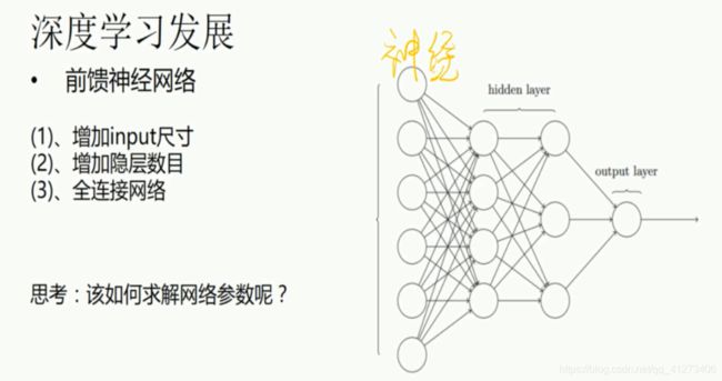
P13.深度学习背景及简介

P14.深度神经网络基础及DNN简介

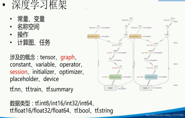
P15.Tensorflow框架简介

P16.Tensorflow入门示例

import tensorflow as tf
import numpy as np

tf.compat.v1.disable_eager_execution()#非常重要
# 用 NumPy 随机生成 100 个数据
x_data = np.float32(np.random.rand(2, 100))
y_data = np.dot([0.100, 0.200], x_data) + 0.300

# 构造一个线性模型
b = tf.Variable(tf.zeros([1]))
W = tf.Variable(tf.random.uniform([1, 2], -1.0, 1.0))
y = tf.matmul(W, x_data) + b

# 最小化方差
loss = tf.reduce_mean(tf.square(y - y_data)) #平均方差
optimizer = tf.compat.v1.train.GradientDescentOptimizer(0.5)#优化器0.5步长
train = optimizer.minimize(loss)
# 初始化变量
init = tf.compat.v1.global_variables_initializer()

# 启动图 (graph)
sess = tf.compat.v1.Session()
sess.run(init)

# 拟合平面
for step in range(0, 201):
    l, _ = sess.run([loss, train])
    print(l)

w_result, b_result = sess.run([W, b])
print(w_result, b_result)

for step in range(0, 201):
    sess.run(train)
    if step % 20 == 0:
        print(step, sess.run(W), sess.run(b))

结果：

因为源码当时的tf版本和现在的版本不同出了一些错误，其中一些小改一下就好了，
但是其中有一个非常坑，找了好久才解决。
地址：https://blog.csdn.net/qq_41273406/article/details/117969984

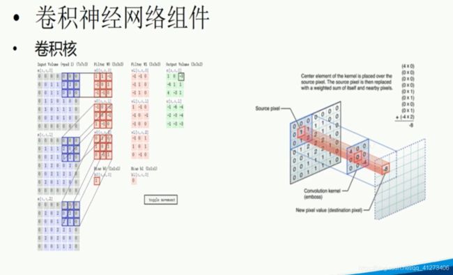
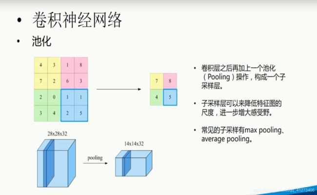
P17.卷积神经网络

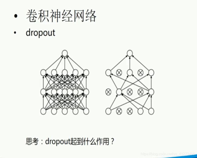
dropout可以减轻过拟合

P18.卷积神经网络代码

这个是课件上的代码，因为版本不同没有运行成功。后面有我自己找到的代码。

from PIL import Image
import tensorflow as tf
from tensorflow.examples.tutorials.mnist import input_data

mnist = input_data.read_data_sets('./MNIST_data', one_hot=True)

# 定义图
x = tf.placeholder(tf.float32, shape=[None, 784]) #接收图像
y_ = tf.placeholder(tf.float32, shape=[None, 10]) #接收标签

x_image = tf.reshape(x, [-1, 28, 28, 1])

#卷积
W_conv1 = tf.Variable(tf.truncated_normal([5, 5, 1, 32], stddev=0.1))#5*5的卷积核，出口1，数量32
b_conv1 = tf.constant(0.1, shape=[32])

h_conv1 = tf.nn.relu(tf.nn.conv2d(x_image, W_conv1, strides=[1, 1, 1, 1], padding='SAME') + b_conv1)#激活函数
h_pool1 = tf.nn.max_pool(h_conv1, ksize=[1, 2, 2, 1], strides=[1, 2, 2, 1], padding='SAME')#池化

#
W_conv2 = tf.Variable(tf.truncated_normal([5, 5, 32, 64], stddev=0.1))
b_conv2 = tf.constant(0.1, shape=[64])

h_conv2 = tf.nn.relu(tf.nn.conv2d(h_pool1, W_conv2, strides=[1, 1, 1, 1], padding='SAME') + b_conv2)
h_pool2 = tf.nn.max_pool(h_conv2, ksize=[1, 2, 2, 1], strides=[1, 2, 2, 1], padding='SAME')

#
W_fc1 = tf.Variable(tf.truncated_normal([7 * 7 * 64, 1024], stddev=0.1))
b_fc1 = tf.constant(0.1, shape=[1024])

h_pool2 = tf.reshape(h_pool2, [-1, 7 * 7 * 64])
h_fc1 = tf.nn.relu(tf.matmul(h_pool2, W_fc1) + b_fc1)

keep_prob = tf.placeholder(tf.float32)
h_fc1 = tf.nn.dropout(h_fc1, keep_prob)

W_fc2 = tf.Variable(tf.truncated_normal([1024, 10], stddev=0.1))
b_fc2 = tf.constant(0.1, shape=[10])

y_conv = tf.matmul(h_fc1, W_fc2) + b_fc2
cross_entropy = tf.reduce_mean(tf.nn.softmax_cross_entropy_with_logits(labels=y_, logits=y_conv))
train_step = tf.train.AdamOptimizer(1e-4).minimize(cross_entropy)
correct_prediction = tf.equal(tf.argmax(y_conv, 1), tf.argmax(y_, 1))
prediction = tf.argmax(y_conv, 1)
accuracy = tf.reduce_mean(tf.cast(correct_prediction, tf.float32))

saver = tf.train.Saver()  # defaults to saving all variables
process_train = False

with tf.Session() as sess:
    if process_train:
        sess.run(tf.global_variables_initializer())
        for i in range(20000):
            batch = mnist.train.next_batch(100)
            _, train_accuracy = sess.run([train_step, accuracy],
                feed_dict={x: batch[0], y_: batch[1], keep_prob: 0.5})
            if i % 100 == 0:
                print("step %d, training accuracy %g" % (i, train_accuracy))

            # 保存模型参数，注意把这里改为自己的路径
            saver.save(sess, './mnist_model/model.ckpt')
            print("test accuracy %g" % accuracy.eval(feed_dict={x: mnist.test.images,
                y_: mnist.test.labels, keep_prob: 1.0}))
    else:
        saver.restore(sess, "./mnist_model/model.ckpt")

    pred_file = "./3.png"
    img_content = Image.open(pred_file)
    img_content = img_content.resize([28, 28])

    pred_content = img_content.convert("1")
    pred_pixel = list(pred_content.getdata())  # get pixel values
    pred_pixel = [(255 - x) * 1.0 / 255.0 for x in pred_pixel]

    pred_num = sess.run(prediction, feed_dict={x: [pred_pixel], keep_prob: 1.0})

    print('recognize result:')
    print(pred_num)

可以运行成功的代码：

https://blog.csdn.net/qq_41273406/article/details/117998232

P19.Word EMbedding模型

P20.循环神经网络 1

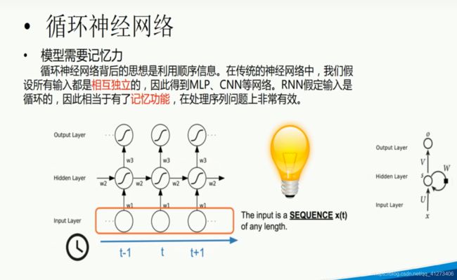
P21.循环神经网络2

P22.循环神经网络应用

23.聊天机器人实战

代码在开头链接中，这个没实现我太菜了。