线性回归 非线性回归
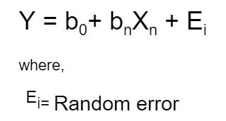
Linear Regression is the most talked-about term for those who are working on ML and statistical analysis. Linear Regression, as the name suggests, simply means fitting a line to the data that establishes a relationship between a target ‘y’ variable with the explanatory ‘x’ variables. It can be characterized by the equation below:
对于从事ML和统计分析的人员来说,线性回归是最受关注的术语。 顾名思义,线性回归只是意味着对数据拟合一条线,以建立目标“ y”变量与解释性“ x”变量之间的关系。 它可以通过以下等式来表征:
Let us take a sample data set which I got from a course on Coursera named “Linear Regression for Business Statistics” .
让我们以示例数据集为例,该数据集是从Coursera上一门名为“业务统计的线性回归”的课程中获得的。
The data set looks like :
数据集如下所示:
Fig-1 图。1The interpretation of the first row is that the first trip took a total of 489.4 minutes to deliver 42 parcels driving through a truck which was 3 years old to a Region B. Here, the time taken is our target variable and ‘Region A’, ‘TruckAge’ and ‘Parcels’ are our explanatory variables. Since, the column ‘Region’ is a categorical variable, it should be encoded with a numeric value.
第一行的解释是,第一次旅行总共花了489.4分钟,通过一辆3岁的卡车将42个包裹运送到B区。在这里,时间是我们的目标变量和“ A区”, “ TruckAge”和“包裹”是我们的解释变量。 由于“区域”列是类别变量,因此应使用数字值对其进行编码。
If we have ‘n’ numbers of labels in our categorical variable then ‘n-1’ extra columns are added to uniquely represent or encode the categorical variable. Here, 1 in RegionA indicates that the trip was to region A and 0 indicates that the trip was to region B.
如果分类变量中有n个标签,则添加n-1个额外的列以唯一表示或编码分类变量。 在此,RegionA中的1表示该行程是到区域A的,0表示该行程是到区域B的。
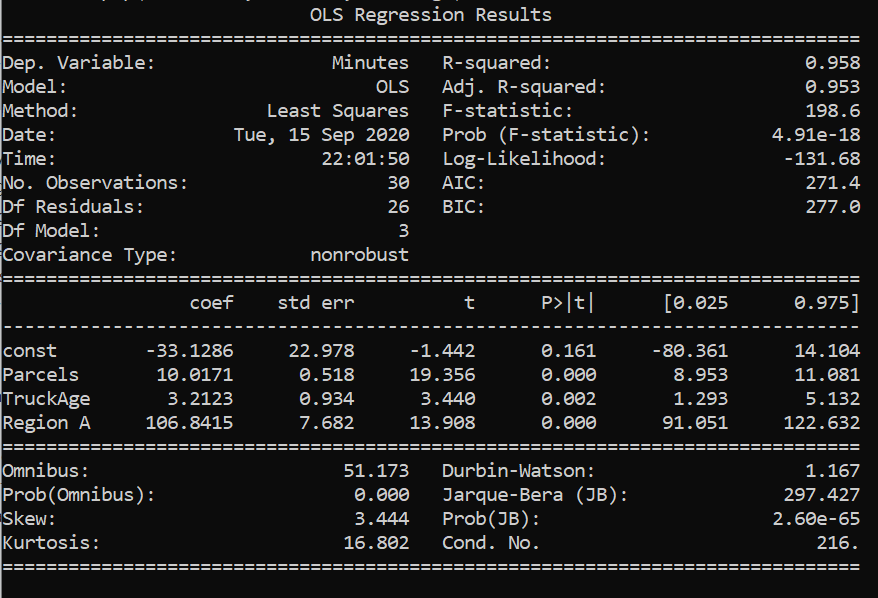
Fig-2 图2Above is the summary of linear regression performed in the data set. Therefore, from the results above, our linear equation would be :
上面是在数据集中执行的线性回归的摘要。 因此,根据以上结果,我们的线性方程为:
Minutes= -33.1286+10.0171*Parcels + 3.21* TruckAge + 106.84* Region A
分钟= -33.1286 + 10.0171 *包裹+ 3.21 * TruckAge + 106.84 *地区A
Interpretation:
解释:
b₁=10.0171: It means that it will take 10.0171 extra minutes to deliver if the number of parcels increases by 1, other variables remaining constant.
b₁= 10.0171:这意味着,这将需要额外的10.0171分钟至递送如果包裹增加1个数,其他变量保持恒定。
b₂=3.21: It means that it will take 3.21 more minutes to deliver if the truck age increases by 1 unit , other variables remaining constant.
b 2 = 3.21:这意味着如果卡车的寿命增加1单位,其他变量保持不变,则要多花3.21分钟。
b₃=106.84: It means that it will take 106.84 more minutes when the delivery is done to Region A as compared with Region B, other variables remaining constant. There’s always a reference variable to compare with when it comes to interpretation of coefficient of a categorical variable and here, the reference is to Region B as we have assigned 0 to region B.
b₃= 106.84:这意味着,当以与区域B中,其他变量保持不变相比,递送做是为了区域A将需要更多106.84分钟。 在解释分类变量的系数时,总是有一个参考变量要与之进行比较。这里,由于我们为区域B分配了0,因此参考区域B。
b₀=-33.1286 : It mathematically means the amount of time taken to deliver 0 parcels by a truck of age 0 to region B. This doesn’t make any sense from a business perspective. Sometimes the intercept may have some meaningful insights to give and sometimes it is just there to fit the data.
b₀= -33.1286:这在数学上指0岁一辆卡车区域B.这提供0包裹不会使从商业角度看任何意义上所花费的时间量。 有时,拦截可能会提供一些有意义的见解,而有时只是为了适应数据。
But, we have to check if this is what defines the relationship between our x variables and y variable. The fit we obtained is an estimate only on a sample data and it is not yet acceptable to conclude that this same relationship may exist on the real data. We must check if the parameters we got are statistically significant or are just there to fit the data to the model. Therefore, it is extremely crucial that we examine the goodness of fit and the significance of the x variables.
但是,我们必须检查这是否定义了x变量和y变量之间的关系。 我们获得的拟合仅是对样本数据的估计,尚不能断定在真实数据上可能存在相同的关系。 我们必须检查获得的参数是否具有统计意义,或者是否正好适合将数据拟合到模型中。 因此,检查拟合优度和x变量的重要性非常关键。
Hypothesis Testing
假设检验
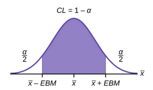
Fig-3, Source: Lumen Learning 图3,来源:流明学习Hypothesis testing can be done by various ways like the t-statistics test, confidence interval test and the p-value test. Here, we’re going to examine the p values corresponding to each of the coefficients.
假设检验可以通过多种方法完成,例如t统计检验,置信区间检验和p值检验。 在这里,我们将检查与每个系数相对应的p值。
For every hypothesis testing, we define a confidence interval i.e (1-alpha), such that this region is called the accepting region and the remaining regions with area alpha/2 on both sides ( in a two tailed test) are the rejection region. In order to do a hypothesis test we must assume a null hypothesis and an alternate hypothesis.
对于每个假设检验,我们定义一个置信区间,即(1-alpha),以使该区域称为接受区域,而两侧(在两个尾部检验中)面积为α/ 2的其余区域为拒绝区域。 为了进行假设检验,我们必须假设一个原假设和另一个假设。
Null Hypothesis : This X variable has no effect on the Y variable i.e H₀: b=0
零假设:此X变量对Y变量无效,即H₀ :b = 0
Alternate Hypothesis: This X variable has effect on the Y variable i.e
替代假设:此X变量对Y变量有影响,即
H₁: b ≠0
H₁ :b ≠ 0
Fig-4 图4Null hypothesis is only accepted if the p-value is greater than the value of alpha/2. As we can see from the table above, all the p values are less than 0.05/2 ( if we take a 95% confidence interval). This means the p value lies somewhere in the rejecting region and therefore, we can reject the null hypothesis. Thus, all of our x variables are important in defining the y variable. And, the coefficient of the x variables are statistically significant and are not there just to fit the data to the model.
仅当p值大于alpha / 2的值时,才接受零假设。 从上表可以看出,所有p值均小于0.05 / 2(如果我们采用95%的置信区间)。 这意味着p值位于拒绝区域中的某个位置,因此,我们可以拒绝原假设。 因此,我们所有的x变量对于定义y变量都很重要。 并且,x变量的系数在统计上是显着的,而不仅仅是为了使数据适合模型。
Our Own hypothesis testing
我们自己的假设检验
The above hypothesis was the default hypothesis done by the statsmodel itself. Lets us assume that we have a popular belief that the amount of time taken to make the delivery increases by 5 minutes with unit increase in the truck age , keeping all other variables constant. Now we can test if this belief still holds in our model.
以上假设是statsmodel本身所做的默认假设。 让我们假设我们普遍认为,随着卡车使用年限的增加,交货时间增加了5分钟,而其他所有变量均保持不变。 现在我们可以测试这种信念是否仍然适用于我们的模型。
Null hypothesis H₀ : b₂=5
零假设H₀:b 2 = 5
Alternate Hypothesis H₁ : b₂ ≠5
替代假设H₁:b 2≠5
The OLS Regression results show that the range of values of the coefficient of TruckAge is : [1.293 , 5.132] . For these values of coefficient, the variable is considered to be statistically significant. The midpoint of the interval [1.293 , 5.132] is our estimated coefficient given by the model. Since our test statistic is 5 minutes and it lies within the range [1.293 , 5.132], we cannot ignore the null hypothesis. Therefore, we cannot ignore the popular belief that it takes extra 5 minutes to deliver through a unit year older truck. In the end, b₂ is taken 3.2123 , its just that the hypothesis is providing enough evidence that the b₂ that we have estimated is a good estimation. However, 5 minutes can also be a possible good estimation of b₂.
OLS回归结果表明,TruckAge系数的取值范围是[1.293,5.132] 。 对于这些系数值,该变量被认为具有统计意义。 区间[1.293,5.132]的中点是模型给出的估计系数。 由于我们的检验统计量是5分钟,并且处于[1.293,5.132]范围内,因此我们不能忽略原假设。 因此,我们不能忽视这样一种普遍的观念,即通过一辆单位年限的旧卡车需要花费额外的5分钟。 最后,将b 2取为3.2123,这恰恰是该假设提供了足够的证据证明我们估计的b 2是一个很好的估计。 但是,5分钟也可能是b 2的良好估计。
Measuring the goodness of fit
衡量合身度
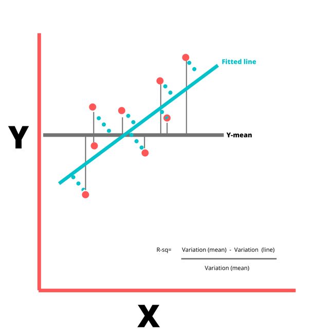
The R square value is used as a measure of goodness of fit. The value 0.958 indicates that 95.8% of variations in Y variable can be explained by our X variables. The remaining variations in Y go unexplained.
R平方值用作拟合优度的度量。 值0.958表示Y变量的95.8%的变化可以由我们的X变量解释。 Y的其余变化无法解释。
Total SS= Regression SS + Residual SS
总SS =回归SS +残留SS
R square= Regression SS/ Total SS
R square =回归SS /总SS
Fig-5, Figure by Author 图5,作者制图Lowest value of R square can be 0 and highest can be 1. A low R-squared value indicates a poor fit and signifies that you might be missing some important explanatory variables. The value of R- square increases by increase in X variables, irrespective of whether the added X variable is important or not. So to adjust with this, there’s Adjusted R square value that increases only if the additional X variable improves the model more than would be expected by chance and decreases when additional variable improves the model by less than expected by chance.
R square的最小值可以为0,最大值可以为1。Rsquared值低表示拟合度差,表示您可能缺少一些重要的解释变量。 R平方的值随X变量的增加而增加,而不管所添加的X变量是否重要。 因此,要对此进行调整,只有当附加X变量对模型的改进超出偶然期望的程度时,“调整后的R平方”值才会增加;而当附加变量对模型的改进小于偶然期望的幅度时,则将减小R平方值。
Residual Plots
残留图
There are some assumptions made about this random error before the linear regression is performed.
在执行线性回归之前,有一些关于此随机误差的假设。
- The mean of the random error is 0 . 随机误差的平均值为0。
- The random errors have a constant variance. 随机误差具有恒定的方差。
- The errors are normally distributed. 错误是正态分布的。
- The error instances are independent of each other 错误实例彼此独立
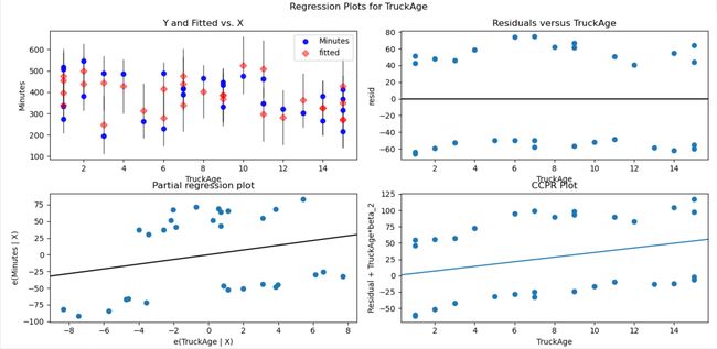
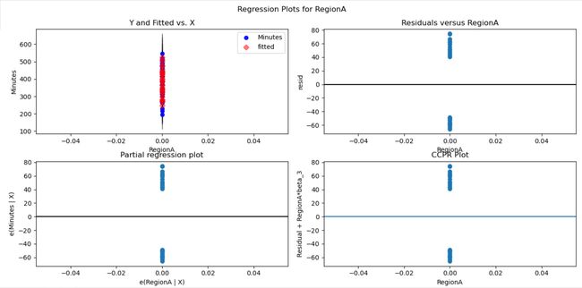
In the plots above, the residuals vs X variable plots show if our model assumptions are violated or not. In fig-6 , the residual vs parcels plot seems to be scattered. The residuals are distributed randomly around zero and seem to have a constant variance. Same is the case with residual plots of the other x variables. Therefore, the initial assumptions about the random error still hold. If there were any curvature/trends among the residuals or the variance seems to be changing with the x variable (or any other dimension) then, it could signify that there’s a huge problem with our linear model as the initial assumptions violated. In such cases, box cox method should be performed. It is a process where the problematic x variable is subjected to transformations like log or square root so that the residue would have a constant variance. The kind of transformation to do with the x variable is like a hit and trial method.
在上面的图中,残差与X变量图显示了是否违反了我们的模型假设。 在图6中,残差与宗地图似乎是分散的。 残差在零附近随机分布,并且似乎具有恒定的方差。 其他x变量的残差图也是如此。 因此,关于随机误差的初始假设仍然成立。 如果残差之间存在任何曲率/趋势,或者方差似乎随着x变量(或任何其他维度)而变化,那么这可能表明线性模型存在巨大问题,因为违反了初始假设。 在这种情况下,应执行Box Cox方法。 在此过程中,将有问题的x变量进行对数或平方根之类的转换,以便残差具有恒定的方差。 使用x变量进行转换的方式类似于点击和试用方法。
Multi-collinearity
多重共线性
Multi-collinearity occurs when there are high correlations among independent variables in a multiple regression model that can causes insignificant p values although the independent variables are tested important individually.
当多元回归模型中的独立变量之间存在高度相关性时,会产生多重共线性,尽管尽管对各个独立变量进行了重要测试,但它们可能导致无关紧要的p值。
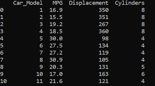
Let us consider the data set :
让我们考虑数据集:
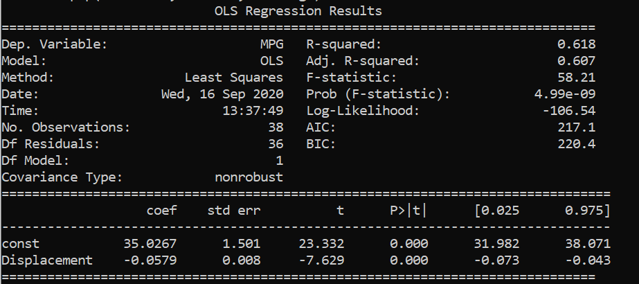
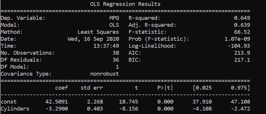
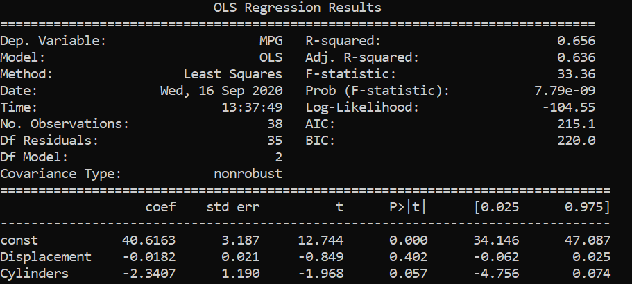
Data set from Linear Regression for Business Statistics-Coursera 来自 商务统计线性拟合的数据集 -Coursera Fitting the data with MPG as our response variable and Displacement as X variable. 用MPG作为我们的响应变量,将Displacement作为X变量拟合数据。 Fitting the data with MPG as our response variable and Cylinders as X variable. 用MPG作为我们的响应变量,将Cylinders作为X变量拟合数据。 Fitting the data with MPG as our response variable and Cylinders and Displacement as X variables. 用MPG拟合数据作为我们的响应变量,将圆柱度和位移拟合为X变量。From the above results, we saw that displacements and cylinders seem to be statistically important variables as their p-values are less than alpha/2 in the first two results where single variable linear regression was performed.
从以上结果可以看出,在执行单变量线性回归的前两个结果中,位移和柱面似乎是统计上重要的变量,因为它们的p值小于alpha / 2。
When multi linear regression was performed, both the x variables turned out to be unimportant as their p-values are greater than alpha/2 . However, both the variables are important as per the previous two simple regressions. This might be caused by multicollinearity in the data set.
当执行多元线性回归时,两个x变量都变得不重要,因为它们的p值大于alpha / 2。 但是,根据前面的两个简单回归,这两个变量都很重要。 这可能是由于 多重共线性 在数据集中。
We can see that the displacement and cylinders are strongly correlated with each other with a correlation coefficient of 0.94. Therefore, to deal with such issues, one of the highly correlated variables should be avoided in linear regression.
我们可以看到,位移和圆柱体之间具有很强的相关性,相关系数为0.94。 因此,为解决此类问题,在线性回归中应避免使用高度相关的变量之一。
The overall code can be found here.
总体代码可以在这里找到。
Thanks for reading!
谢谢阅读!
翻译自: https://medium.com/@paridhiparajuli/interpretation-of-linear-regression-dba45306e525
线性回归 非线性回归

