[TensorFlow系列-9]：TensorFlow基础 - 张量元素的统计运算

 作者主页(文火冰糖的硅基工坊)：https://blog.csdn.net/HiWangWenBing

本文网址：https://blog.csdn.net/HiWangWenBing/article/details/119636601

---

目录

第1章 Tensor运算概述

1.1 概述

1.3  “in place“运算: 不支持

1.4 Tensor的广播机制: 不同维度的tensor实例运算

1.5 环境准备

1.6 统计运算概述

第2章 降维求平均值：tf.reduce_mean(input_tensor, axis=None)

第3章 降维求汇总值：tf.reduce_sum(input_tensor, axis=None)

第4章 降维求乘积：tf.reduce_prod(input_tensor, axis=None)

第5章 降维求最大值：tf.reduce_max(input_tensor, axis=None)

第6章 降维求最小值：tf.reduce_min(input_tensor, axis=None,)

第7章 降维逻辑与：tf.reduce_all(input_tensor, axis=None)

第8章 降维逻辑或：tf.reduce_any(input_tensor, axis=None)

第9章 最大值索引：tf.argmax(input_tensor, axis=None)

最10章 最小值索引：tf.argmin(input_tensor, axis=None)

第11章 中位数Median：NA

第12章 众数值mode： NA

第13章 标准方差std：NA

第14章 方差var：NA

第15章 频度bincount：NA

---

第1章 Tensor运算概述

1.1 概述

TensorFlow提供了大量的张量运算，基本上可以对标Numpy多维数组的运算，以支持对张量的各种复杂的运算。

这些操作运算中大多是对数组中每个元素执行相同的函数运算，并获得每个元素函数运算的结果序列，这些序列生成一个新的同维度的数组。

https://www.w3cschool.cn/tensorflow_python/tensorflow_python-4ihe2hen.html

1.2 运算分类

（1）算术运算：加、减、系数乘、系数除

（2）函数运算：sin，cos

（3）取整运算：上取整、下取整

（4）统计运算：最大值、最小值、均值

（5）线性代数运算：矩阵、点乘、叉乘

1.3  “in place“运算: 不支持

1.4 Tensor的广播机制: 不同维度的tensor实例运算

1.5 环境准备

#环境准备
import numpy as np
import tensorflow as tf
print("hello world")
print("tensorflow version:", tf.__version__)

1.6 统计运算概述

Tensorflow提供了很多统计函数，用于从Tensor中查找最小元素，最大元素等。

第2章 降维求平均值：tf.reduce_mean(input_tensor, axis=None)

（1）原理概述

算术平均值是沿轴的元素的总和除以元素的数量。

算术平均值平均的前提是：求出所有带符号数值的总和。

简单算术平均公式：

设一组数据为X1，X2，...，Xn，简单的算术平均数的计算公式为：

（2） 函数使用说明

mean() 函数返回数组中元素的算术平均值。 如果提供了轴，则沿其计算。

 （3）案例

• 全统计

# 求所有元素的算术平均值

a = tf.constant([[1,2,3],[4,5,6]])  
print ("源数据：")
print (a)

print ("\n结果数据：")
print (tf.reduce_mean(a)) 
# print (a.mean()) # 不支持

输出：

源数据：
tf.Tensor(
[[1 2 3]
 [4 5 6]], shape=(2, 3), dtype=int32)

结果数据：
tf.Tensor(3, shape=(), dtype=int32)

• 按列统计（axis=0方向）

# 按列求算术平均值

a = tf.constant([[1.,2.,3.],[4.,5.,6.]])  
print ("源数据：")
print (a)


print ("\n结果数据：")
print (tf.reduce_mean(a,axis=0)) 

输出：

源数据：
tf.Tensor(
[[1. 2. 3.]
 [4. 5. 6.]], shape=(2, 3), dtype=float32)

结果数据：
tf.Tensor([2.5 3.5 4.5], shape=(3,), dtype=float32)

结果数据：
tf.Tensor([2. 5.], shape=(2,), dtype=float32)

• 按行方向（dim=1）

# 按行求算术平均值

a = tf.constant([[1.0,2.0,3],[4.,5.,6.]])  
print ("源数据：")
print (a)

print ("\n结果数据：")
print (tf.reduce_mean(a,axis=1)) 

输出：

源数据：
tf.Tensor(
[[1. 2. 3.]
 [4. 5. 6.]], shape=(2, 3), dtype=float32)

结果数据：
tf.Tensor([2. 5.], shape=(2,), dtype=float32)

---

第3章 降维求汇总值：tf.reduce_sum(input_tensor, axis=None)

sum求出所有元素的算术和。

（1）全统计

# 求所有元素的算术和

a = tf.constant([[1,2,3],[4,5,6]])  
print ("源数据：")
print (a)

print ("\n结果数据：")
print (tf.reduce_sum(a)) 
# print (a.sum())  #不支持

输出：

源数据：
tf.Tensor(
[[1 2 3]
 [4 5 6]], shape=(2, 3), dtype=int32)

结果数据：
tf.Tensor(21, shape=(), dtype=int32)

（2）按列统计（按照dim=0方向）

# 求所有元素的算术和

a = tf.constant([[1,2,3],[4,5,6]])  
print ("源数据：")
print (a)

print ("\n结果数据(axis=0)：")
print (tf.reduce_sum(a,axis=0)) 
#  print (a.reduce_sum(axis=0))  # 不支持

输出：

源数据：
tf.Tensor(
[[1 2 3]
 [4 5 6]], shape=(2, 3), dtype=int32)

结果数据(axis=0)：
tf.Tensor([5 7 9], shape=(3,), dtype=int32)

（3）按行统计（按照dim=1方向）

# 求所有元素的算术和

a = tf.constant([[1,2,3],[4,5,6]])  
print ("源数据：")
print (a)

print ("\n结果数据(axis=1)：")
print (tf.reduce_sum(a,axis=1)) 
# print (a.sum(dim=1)) # 不支持

输出：

源数据：
tf.Tensor(
[[1 2 3]
 [4 5 6]], shape=(2, 3), dtype=int32)

结果数据(axis=1)：
tf.Tensor([ 6 15], shape=(2,), dtype=int32)

---

第4章 降维求乘积：tf.reduce_prod(input_tensor, axis=None)

prod()函数用来计算所有元素的乘积。

输出：

源数据：
tensor([[1., 2., 3.],
        [4., 5., 6.]])


结果数据：
tensor(720.)
tensor(720.)

输出结果：

源数据：

tensor([[1., 2., 3.],
        [4., 5., 6.]])


结果数据：
tensor(720.)
tensor(720.)

第5章 降维求最大值：tf.reduce_max(input_tensor, axis=None)

max（）找出所有元素中，算术值最大的数值。

# 求所有元素的最大值

a = tf.constant([[1,2,3],[4,5,6]])  
print ("源数据：")
print (a)

print ("\n结果数据：")
b = tf.reduce_max(a)
print (b) 
# print(a.max)  # 不支持

源数据：
tf.Tensor(
[[1 2 3]
 [4 5 6]], shape=(2, 3), dtype=int32)

结果数据：
tf.Tensor(6, shape=(), dtype=int32)

第6章 降维求最小值：tf.reduce_min(input_tensor, axis=None,)

min（）找出所有元素中，算术值最小的数值。

# 求所有元素的最小值

a = tf.constant([[1,2,3],[4,5,0]])  
print ("源数据：")
print (a)

print ("\n结果数据：")
b = tf.reduce_min(a)
print (b) 
#print (a.min()) 

输出：

源数据：
tf.Tensor(
[[1 2 3]
 [4 5 0]], shape=(2, 3), dtype=int32)

结果数据：
tf.Tensor(0, shape=(), dtype=int32)

第7章 降维逻辑与：tf.reduce_all(input_tensor, axis=None)

逻辑与：所有元素为true，输出就为true

# 源代码示例
# 求逻辑和（“与”）
a = tf.constant([[True,True,True],[True,False,False]])  
print ("源数据：")
print (a)

print ("结果数据：")
print (tf.reduce_all(a))
print (tf.reduce_all(a,axis=0)) 
print (tf.reduce_all(a,axis=1)) 

输出：

源数据：
tf.Tensor(
[[ True  True  True]
 [ True False False]], shape=(2, 3), dtype=bool)
结果数据：
tf.Tensor(False, shape=(), dtype=bool)
tf.Tensor([ True False False], shape=(3,), dtype=bool)
tf.Tensor([ True False], shape=(2,), dtype=bool)

第8章 降维逻辑或：tf.reduce_any(input_tensor, axis=None)

逻辑或：任意一个为true，输出就为true

# 代码示例

# 求逻辑“或”
a = tf.constant([[True,False,True],[True,False,False]])  
print ("源数据：")
print (a)

print ("结果数据：")
print (tf.reduce_any(a))
print (tf.reduce_any(a,axis=0)) 
print (tf.reduce_any(a,axis=1)) 

输出：

源数据：
tf.Tensor(
[[ True False  True]
 [ True False False]], shape=(2, 3), dtype=bool)
结果数据：
tf.Tensor(True, shape=(), dtype=bool)
tf.Tensor([ True False  True], shape=(3,), dtype=bool)
tf.Tensor([ True  True], shape=(2,), dtype=bool)

第9章 最大值索引：tf.argmax(input_tensor, axis=None)

argmax求所有元素中最大值的索引,index从0开始，线性排列。

# 求所有元素中最大值的索引,index从0开始，线性排列

a = tf.constant([[7,3,5,1],[2,8,4,6]])  
print ("源数据：")
print (a)

print ("\n结果数据(axis=None)：")
print (tf.argmax(a)) 

print ("\n结果数据(axis=0)：")
print (tf.argmax(a,axis=0)) 

print ("\n结果数据(axis=1)：")
print (tf.argmax(a,axis=1)) 
#print (a.argmax()) 

输出：

源数据：
tf.Tensor(
[[7 3 5 1]
 [2 8 4 6]], shape=(2, 4), dtype=int32)

结果数据(axis=None)：
tf.Tensor([0 1 0 1], shape=(4,), dtype=int64)

结果数据(axis=0)：
tf.Tensor([0 1 0 1], shape=(4,), dtype=int64)

结果数据(axis=1)：
tf.Tensor([0 1], shape=(2,), dtype=int64)

最10章 最小值索引：tf.argmin(input_tensor, axis=None)

# 求所有元素中最小值的索引,index从0开始，线性排列

a = torch.Tensor([[1,2,3,4],[5,6,7,8]])   
print ("源数据：")
print (a)
print ('\n')


print ("结果数据：")
print (torch.argmin(a)) 
print (a.argmin()) 

输出：

源数据：
tensor([[1., 2., 3., 4.],
        [5., 6., 7., 8.]])


结果数据：
tensor(0)
tensor(0)

第11章 中位数Median：NA

中位数（Median）又称中值，统计学中的专有名词，是按顺序排列的一组数据中居于中间位置的数（不是数值平均），代表一个样本、种群或概率分布中的一个数值，其可将数值集合划分为相等的上下两部分。

对于有限的数集，可以通过把所有观察值高低排序后找出正中间的一个作为中位数。

如果观察值有偶数个，通常取最中间的两个数值的平均数作为中位数。

第12章 众数值mode： NA

众数（Mode）是指在统计分布上具有明显集中趋势点的数值，代表数据的一般水平。 也是一组数据中出现次数最多的数值，有时众数在一组数中有好几个。

众数是样本观测值在频数分布表中频数最多的那一组的组中值，主要应用于大面积普查研究之中。

众数是在一组数据中,出现次数最多的数据，是一组数据中的原数据，而不是相应的次数。

一组数据中的众数不止一个，如数据2、3、-1、2、1、3中，2、3都出现了两次，它们都是这组数据中的众数。

一般来说，一组数据中，出现次数最多的数就叫这组数据的众数。

例如：1，2，3，3，4的众数是3。

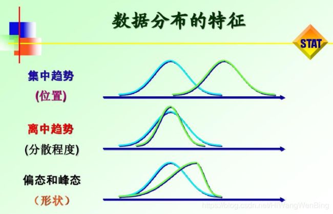
第13章 标准方差std：NA

（1）理论概述

标准差是一组数据离平均值的分散程度的一种度量。

标准差（Standard Deviation） ，是离均差平方的算术平均数（即：方差）的算术平方根，用σ表示。

标准差也被称为标准偏差，或者实验标准差，在概率统计中最常使用作为统计分布程度上的测量依据。

 

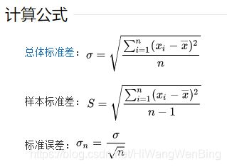
 在实验中单次测量总是难免会产生误差，为此我们经常测量多次，然后用测量值的平均值表示测量的量，并用误差条来表征数据的分布，其中误差条的高度为±标准误差。这里即标准差。

 

如果数组是 [1，2，3，4]，则其平均值为 2.5。 因此，差的平方是 [2.25,0.25,0.25,2.25]，并且再求其平均值的平方根除以 4，即 sqrt(5/4) ，结果为 1.1180339887498949。

第14章 方差var：NA

（1）概述

统计中的方差（样本方差）是每个样本值与全体样本值的平均数之差的平方值的平均数，即 mean((x - x.mean())** 2)。 #mean：求平均

换句话说，标准差是方差的平方根

（2）方差与标准方差的关系：

备注：正态分布使用的是标准方差，而不是方差。

第15章 频度bincount：NA

bincount求你所有元素出现的次数.

---

作者主页(文火冰糖的硅基工坊)：https://blog.csdn.net/HiWangWenBing

本文网址：https://blog.csdn.net/HiWangWenBing/article/details/119636601