1.Introduction: Hands-on Graph Neural Networks

       PyG（PyTorch Geometric）是一个基于PyTorch的库，用于轻松编写和训练图形神经网络（GNN），用于与结构化数据相关的广泛应用。博客好久没有更新了，恰逢1024创作纪念日，浅浅更新一下吧。

       这个是PyG的官网教程，所有代码我都加了注释，最开始我计划翻译一下，但感觉翻译出来很多东西都变味啦，所以保留了英文。后续可能会在B站录制视频，大家有问题可以留言。

       安装环境我这里就不多说啦，我们下面就正式进入PyG的学习。

import os
import torch
os.environ['TORCH'] = torch.__version__

# 这行代码意思是将环境变量中名为'TORCH'的变量设为当前正在运行的PyTorch版本号。

# 具体来说，os.environ 是Python内置的一个标准库，它提供了一个字典类型的接口，用于访问操作系统的环境变量。
# 在这个例子中，os.environ 字典中的 'TORCH' 键被设置为了 torch.__version__ 的值，即当前安装的PyTorch库的版本号。

# 这行代码的目的可能是在代码运行时检查当前系统中安装的PyTorch版本，并将其保存到环境变量中，以便其他代码可以轻松地访问该信息。

这里显示了我安装的PyTorch版本：

Introduction: Hands-on Graph Neural Networks

       Recently, deep learning on graphs has emerged to one of the hottest research fields in the deep learning community.
       Here, Graph Neural Networks (GNNs) aim to generalize classical deep learning concepts to irregular structured data (in contrast to images or texts) and to enable neural networks to reason about objects and their relations.

       This is done by following a simple neural message passing scheme, where node features ${\mathbf{x}}_v^{(\ell )}$ of all nodes $v\in \mathcal{V}$ in a graph $\mathcal{G}=(\mathcal{V},\mathcal{E})$ are iteratively updated by aggregating localized information from their neighbors $\mathcal{N}(v)$:

$${\mathbf{x}}_v^{(\ell +1)}=f_{\theta }^{(\ell +1)}\left({\mathbf{x}}_v^{(\ell )},\left\{{\mathbf{x}}_w^{(\ell )}:w\in \mathcal{N}(v)\right\}\right)$$

       This tutorial will introduce you to some fundamental concepts regarding deep learning on graphs via Graph Neural Networks based on the PyTorch Geometric (PyG) library.
       PyTorch Geometric is an extension library to the popular deep learning framework PyTorch, and consists of various methods and utilities to ease the implementation of Graph Neural Networks.

       Following Kipf et al. (2017), let’s dive into the world of GNNs by looking at a simple graph-structured example, the well-known Zachary’s karate club network.
       This graph describes a social network of 34 members of a karate club and documents links between members who interacted outside the club. Here, we are interested in detecting communities that arise from the member’s interaction.

       PyTorch Geometric provides an easy access to this dataset via the torch_geometric.datasets subpackage:

from torch_geometric.datasets import KarateClub

dataset = KarateClub()
print(f'Dataset: {dataset}:')
print('======================')
print(f'Number of graphs: {len(dataset)}')
print(f'Number of features: {dataset.num_features}')
print(f'Number of classes: {dataset.num_classes}')

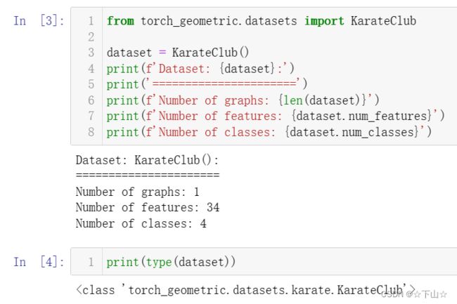
       After initializing the KarateClub dataset, we first can inspect some of its properties.

       For example, we can see that this dataset holds exactly one graph, and that each node in this dataset is assigned a 34-dimensional feature vector (which uniquely describes the members of the karate club).
       Furthermore, the graph holds exactly 4 classes, which represent the community each node belongs to.

       Let’s now look at the underlying graph in more detail:

data = dataset[0]  # Get the first graph object.

print(data)
print('==============================================================')

# Gather some statistics about the graph.
print(f'Number of nodes: {data.num_nodes}')
print(f'Number of edges: {data.num_edges}')
print(f'Average node degree: {data.num_edges / data.num_nodes:.2f}')
print(f'Number of training nodes: {data.train_mask.sum()}') # 4个节点有标签
print(f'Training node label rate: {int(data.train_mask.sum()) / data.num_nodes:.2f}')
print(f'Has isolated nodes: {data.has_isolated_nodes()}') # 孤立节点
print(f'Has self-loops: {data.has_self_loops()}')
print(f'Is undirected: {data.is_undirected()}') # 无向图

print(type(data))

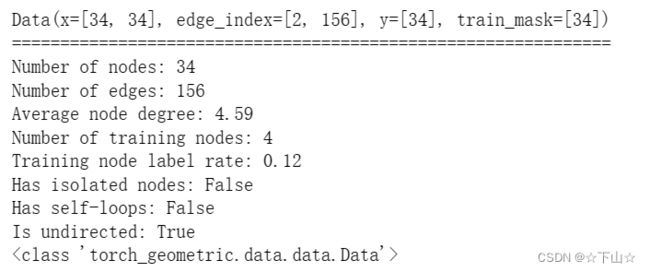
       Each graph in PyTorch Geometric is represented by a single Data object, which holds all the information to describe its graph representation.
       We can print the data object anytime via print(data) to receive a short summary about its attributes and their shapes:

Data(edge_index=[2, 156], x=[34, 34], y=[34], train_mask=[34])

       We can see that this data object holds 4 attributes:
       (1) The edge_index property holds the information about the graph connectivity, i.e., a tuple of source and destination node indices for each edge.
       PyG further refers to (2) node features as x (each of the 34 nodes is assigned a 34-dim feature vector), and to (3) node labels as y (each node is assigned to exactly one class).
       (4) There also exists an additional attribute called train_mask, which describes for which nodes we already know their community assigments.
       In total, we are only aware of the ground-truth labels of 4 nodes (one for each community), and the task is to infer the community assignment for the remaining nodes.

       The data object also provides some utility functions to infer some basic properties of the underlying graph.
       For example, we can easily infer whether there exists isolated nodes in the graph (i.e. there exists no edge to any node), whether the graph contains self-loops (i.e., $(v,v)\in \mathcal{E}$), or whether the graph is undirected (i.e., for each edge $(v,w)\in \mathcal{E}$ there also exists the edge $(w,v)\in \mathcal{E}$).

       Let us now inspect the edge_index property in more detail:


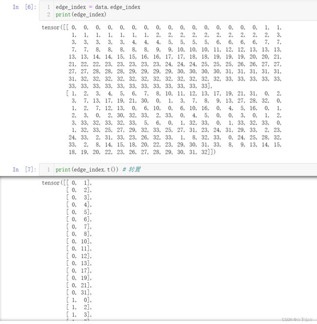
       By printing edge_index, we can understand how PyG represents graph connectivity internally.
We can see that for each edge, edge_index holds a tuple of two node indices, where the first value describes the node index of the source node and the second value describes the node index of the destination node of an edge.

       This representation is known as the COO format (coordinate format) commonly used for representing sparse matrices.
       Instead of holding the adjacency information in a dense representation $\mathbf{A}\in \{0,1{\}}^{|\mathcal{V}|\times |\mathcal{V}|}$, PyG represents graphs sparsely, which refers to only holding the coordinates/values for which entries in $\mathbf{A}$ are non-zero.

       Importantly, PyG does not distinguish between directed and undirected graphs, and treats undirected graphs as a special case of directed graphs in which reverse edges exist for every entry in edge_index.

       We can further visualize the graph by converting it to the networkx library format, which implements, in addition to graph manipulation functionalities, powerful tools for visualization:

# 可视化图
%matplotlib inline
import networkx as nx
import matplotlib.pyplot as plt

def visualize_graph(G, color):
    plt.figure(figsize=(7,7)) # (7, 7)的画布
    plt.xticks([]) # x轴刻度
    plt.yticks([]) # y轴刻度
    nx.draw_networkx(G, pos=nx.spring_layout(G, seed=42), with_labels=True, node_color=color, cmap="Set2")
    
#     其中，G 是一个 NetworkX 图形对象，它可以是一个无向图或有向图。
#     pos 参数表示节点的布局位置，它可以是一个字典，指定每个节点的坐标位置，
#     也可以是一个函数，用于自动计算节点的坐标位置。
#     在这个例子中，使用 nx.spring_layout(G, seed=42) 函数自动计算节点的坐标位置，
#     其中 seed 参数用于指定随机数种子，以确保结果可重复。
#     with_labels 参数表示是否在节点上显示标签，默认为 False，即不显示标签。
#     node_color 参数表示节点的颜色，可以是一个单一的颜色值，也可以是一个颜色列表，指定每个节点的颜色。
#     在这个例子中，使用了一个颜色列表 color，它与节点数量相同，表示每个节点的颜色。
#     cmap 参数表示使用的颜色映射，用于将节点颜色映射到颜色列表中的颜色。在这个例子中，使用了颜色映射 "Set2"。

    plt.show()
    
from torch_geometric.utils import to_networkx

G = to_networkx(data, to_undirected=True)

# to_networkx(data, to_undirected=True) 是 NetworkX 库中用于将图形数据转换为 NetworkX 图形对象的函数之一。
# 其中，data 参数是要转换的数据，它可以是多种格式，如邻接矩阵、边列表、邻接列表等等。
# 具体来说，如果 data 是邻接矩阵，则需要使用 nx.from_numpy_matrix() 函数；
# 如果 data 是边列表或邻接列表，则可以使用 nx.from_edgelist() 或 nx.from_adjacency_list() 函数。

visualize_graph(G, color=data.y)

Implementing Graph Neural Networks

       After learning about PyG’s data handling, it’s time to implement our first Graph Neural Network!

       For this, we will use on of the most simple GNN operators, the GCN layer (Kipf et al. (2017)), which is defined as

$${\mathbf{x}}_v^{(\ell +1)}={\mathbf{W}}^{(\ell +1)}\sum _{w\in \mathcal{N}(v)\cup \{v\}}\frac{1}{c_{w,v}}\cdot {\mathbf{x}}_w^{(\ell )}$$

       where ${\mathbf{W}}^{(\ell +1)}$ denotes a trainable weight matrix of shape [num_output_features, num_input_features] and $c_{w,v}$ refers to a fixed normalization coefficient for each edge.

       PyG implements this layer via GCNConv, which can be executed by passing in the node feature representation x and the COO graph connectivity representation edge_index.

       With this, we are ready to create our first Graph Neural Network by defining our network architecture in a torch.nn.Module class:

import torch
from torch.nn import Linear
from torch_geometric.nn import GCNConv


class GCN(torch.nn.Module):
    def __init__(self):
        super().__init__()
#         torch.manual_seed(1234)
#         torch.manual_seed(1234)的作用是设置随机数生成器的种子(seed)为1234，
#         以确保随机数生成器生成的随机数序列是可重复的。
#         在使用深度学习模型时，通常需要随机初始化模型参数、划分数据集等操作，这些操作都需要使用随机数。
#         设置种子可以确保每次程序运行时生成的随机数序列都是相同的，
#         这样可以使得实验的结果更加可重复，便于调试和比较不同模型的性能。
#         在 PyTorch 中，随机数生成器有多个，包括全局随机数生成器和每个模块自己的随机数生成器。
#         使用 torch.manual_seed() 可以设置全局随机数生成器的种子，而对于每个模块自己的随机数生成器，
#         可以通过创建一个新的 torch.Generator 对象并设置其种子来实现随机数的可重复性。

        self.conv1 = GCNConv(dataset.num_features, 4)
        self.conv2 = GCNConv(4, 4)
        self.conv3 = GCNConv(4, 2)
        self.classifier = Linear(2, dataset.num_classes)

    def forward(self, x, edge_index):
        h = self.conv1(x, edge_index)
        h = h.tanh()
        h = self.conv2(h, edge_index)
        h = h.tanh()
        h = self.conv3(h, edge_index)
        h = h.tanh()  # Final GNN embedding space.
        
        # Apply a final (linear) classifier.
        out = self.classifier(h)

        return out, h

model = GCN()
print(model)

       Here, we first initialize all of our building blocks in __init__ and define the computation flow of our network in forward.
       We first define and stack three graph convolution layers, which corresponds to aggregating 3-hop neighborhood information around each node (all nodes up to 3 “hops” away).
       In addition, the GCNConv layers reduce the node feature dimensionality to $2$, i.e., $34\to 4\to 4\to 2$. Each GCNConv layer is enhanced by a tanh non-linearity.

       After that, we apply a single linear transformation (torch.nn.Linear) that acts as a classifier to map our nodes to 1 out of the 4 classes/communities.

       We return both the output of the final classifier as well as the final node embeddings produced by our GNN.
       We proceed to initialize our final model via GCN(), and printing our model produces a summary of all its used sub-modules.

Embedding the Karate Club Network

       Let’s take a look at the node embeddings produced by our GNN.
       Here, we pass in the initial node features x and the graph connectivity information edge_index to the model, and visualize its 2-dimensional embedding.

def visualize_embedding(h, color, epoch=None, loss=None):
    plt.figure(figsize=(7,7))
    plt.xticks([])
    plt.yticks([])
    h = h.detach().cpu().numpy()
    
#     这行代码的作用是将张量h从计算图中分离（detach），并将其转换为NumPy数组（numpy()），最后将其从所在设备中移动到CPU上（cpu()）。
#     分离操作是将张量从当前计算图中分离出来，使得该张量的计算不会对计算图中其他节点的梯度传播产生影响。
#     这通常用于获取模型的中间输出，以便进行后续的计算和处理，而不会影响模型的反向传播。
#     转换为NumPy数组则是将张量对象转换为NumPy数组对象，以便进行各种NumPy操作。
#     将其从设备上移动到CPU上，则是将张量从GPU等计算设备上转移到CPU上，以便进行后续的操作或输出。

    plt.scatter(h[:, 0], h[:, 1], s=140, c=color, cmap="Set2") # 散点图：取第0列；取第一列。散点大小140
    if epoch is not None and loss is not None:
        plt.xlabel(f'Epoch: {epoch}, Loss: {loss.item():.4f}', fontsize=16) # 字体大小16
    plt.show()

model = GCN()

_, h = model(data.x, data.edge_index)
print(h[0:3])
print(f'Embedding shape: {list(h.shape)}')

visualize_embedding(h, color=data.y)

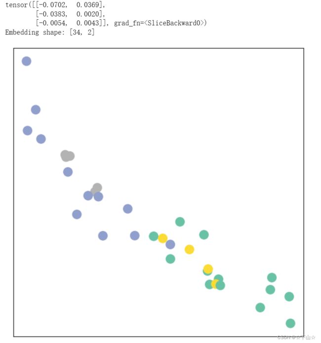
       Remarkably, even before training the weights of our model, the model produces an embedding of nodes that closely resembles the community-structure of the graph.
       Nodes of the same color (community) are already closely clustered together in the embedding space, although the weights of our model are initialized completely at random and we have not yet performed any training so far!
       This leads to the conclusion that GNNs introduce a strong inductive bias, leading to similar embeddings for nodes that are close to each other in the input graph.

Training on the Karate Club Network

       But can we do better? Let’s look at an example on how to train our network parameters based on the knowledge of the community assignments of 4 nodes in the graph (one for each community):

       Since everything in our model is differentiable and parameterized, we can add some labels, train the model and observse how the embeddings react.
       Here, we make use of a semi-supervised or transductive learning procedure: We simply train against one node per class, but are allowed to make use of the complete input graph data.

       Training our model is very similar to any other PyTorch model.
       In addition to defining our network architecture, we define a loss critertion (here, CrossEntropyLoss) and initialize a stochastic gradient optimizer (here, Adam).
       After that, we perform multiple rounds of optimization, where each round consists of a forward and backward pass to compute the gradients of our model parameters w.r.t. to the loss derived from the forward pass.
If you are not new to PyTorch, this scheme should appear familar to you.
Otherwise, the PyTorch docs provide a good introduction on how to train a neural network in PyTorch.

       Note that our semi-supervised learning scenario is achieved by the following line:

loss = criterion(out[data.train_mask], data.y[data.train_mask])

       While we compute node embeddings for all of our nodes, we only make use of the training nodes for computing the loss.
       Here, this is implemented by filtering the output of the classifier out and ground-truth labels data.y to only contain the nodes in the train_mask.

       Let us now start training and see how our node embeddings evolve over time (best experienced by explicitely running the code):

model = GCN()
criterion = torch.nn.CrossEntropyLoss()  # Define loss criterion.
optimizer = torch.optim.Adam(model.parameters(), lr=0.01)  # Define optimizer.

def train(data):
    optimizer.zero_grad()  # Clear gradients.
    out, h = model(data.x, data.edge_index)  # Perform a single forward pass.
    loss = criterion(out[data.train_mask], data.y[data.train_mask])  # Compute the loss solely based on the training nodes.
    loss.backward()  # Derive gradients.
    optimizer.step()  # Update parameters based on gradients.
    return loss, h

for epoch in range(401):
    loss, h = train(data)
    if epoch % 40 == 0:
        visualize_embedding(h, color=data.y, epoch=epoch, loss=loss)

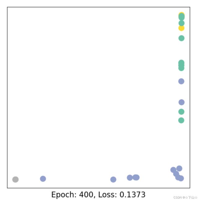
       As one can see, our 3-layer GCN model manages to linearly separating the communities and classifying most of the nodes correctly.

       Furthermore, we did this all with a few lines of code, thanks to the PyTorch Geometric library which helped us out with data handling and GNN implementations.

Conclusion

       This concludes the first introduction into the world of GNNs and PyTorch Geometric.
       In the follow-up sessions, you will learn how to achieve state-of-the-art classification results on a number of real-world graph datasets.

本文内容参考：PyG官网