PyTorch RNN的原理及其手写复现。
PyTorch RNN的原理及其手写复现。
- 0、前言
- 代码实现
-
- 记忆单元(考虑过去的信息)分类包括:1.RNN 2.GRU 3.LSTM
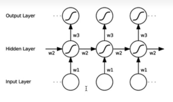
- 模型类别:1.单向循环(左到右) 2.双向循环(考虑未来信息) 3.多层单向或双向循环
- 优缺点
- 应用场景
- 具体公式
0、前言
先给出代码的实现(包括官方API和手动实现)然后逐步介绍RNN的优缺点,应用场景等。
在看代码之前有必要了解输入输出有哪些,以及他们的特性。
官方教程在:
https://pytorch.org/docs/stable/generated/torch.nn.RNN.html#torch.nn.RNN
参数:(实例化时候可以传入的参数)
input_size- 输入 x 中预期特征的数量。hidden_size- 隐藏状态h的特征数。num_layers- 循环层数。例如,设置num_layers=2意味着将两个 RNN 堆叠在一起形成堆叠式 RNN,第二个 RNN 接收第一个 RNN 的输出并计算最终结果。默认值:1nonlinearity- 使用的非线性。可以是tanh或relu。默认值:tanhbias- 如果为False,则该层不使用偏置权重 b_ih 和 b_hh。默认值:Truebatch_first- 如果为True,则输入和输出张量将作为 (batch, seq, feature) 而不是 (seq, batch, feature) 提供。请注意,这不适用于隐藏状态或细胞状态。有关详细信息,请参阅下面的输入/输出部分。默认值:Falsedropout- 如果非零,则在除最后一层之外的每个 RNN 层的输出上引入一个 Dropout 层,dropout 概率等于dropout。默认值:0bidirectional- 如果为True,则成为双向 RNN。默认值:False
输入:(需要初始化的值)
input:对于非批处理输入,形状为 ( L , H i n ) (L, H_{in}) (L,Hin) 的张量, ( L , N , H i n ) (L, N, H_{in}) (L,N,Hin)当batch_first=False或 ( N , L , H i n ) ( N, L, H_{in}) (N,L,Hin) 当batch_first=True时包含输入序列的特征。输入也可以是打包的可变长度序列。有关详细信息,请参阅torch.nn.utils.rnn.pack_padded_sequence()或torch.nn.utils.rnn.pack_sequence()。h_0:形状张量 ( D ∗ num_layers , H o u t ) (D * \text{num\_layers}, H_{out}) (D∗num_layers,Hout) 对于非批处理输入或 ( D ∗ num_layers , N , H o u t ) (D * \text{num\_layers}, N, H_{out}) (D∗num_layers,N,Hout)包含输入序列批次的初始隐藏状态。如果未提供,则默认为零。
其中:
N = b a t c h s i z e L = s e q u e n c e l e n g t h D = 2 i f b i d i r e c t i o n a l = T r u e o t h e r w i s e 1 H i n = i n p u t _ s i z e H o u t = h i d d e n _ s i z e N=batch\ size\\ L=sequence\ length\\ D=2\ if\ bidirectional=True\ otherwise\ 1\\ H_{in}=input\_size\\ H_{out}=hidden\_size N=batch sizeL=sequence lengthD=2 if bidirectional=True otherwise 1Hin=input_sizeHout=hidden_size
输出:output:形状张量 ( L , D ∗ H o u t ) (L, D * H_{out}) (L,D∗Hout) 对于非批处理输入, ( L , N , D ∗ H o u t ) (L, N, D * H_{out} ) (L,N,D∗Hout) 当batch_first=False或 ( N , L , D ∗ H o u t ) (N, L, D * H_{out}) (N,L,D∗Hout) 当batch_first=True对于每个 t,包含来自 RNN 最后一层的输出特征 (h_t)。如果torch.nn.utils.rnn.PackedSequence已作为输入给出,输出也将是一个打包序列。h_n:形状张量 ( D ∗ n u m _ l a y e r s , H o u t ) (D * num\_layers, H_{out}) (D∗num_layers,Hout) 对于非批处理输入或 ( D ∗ n u m _ l a y e r s , N , H o u t ) (D∗num\_layers,N,Hout) (D∗num_layers,N,Hout)包含批次中每个元素的最终隐藏状态。(其实output的最后一个元素就是h_n)
变量:
weight_ih_l[k]- 第 k 层的可学习输入隐藏权重,形状为 (hidden_size, input_size) for k = 0。否则,形状为 (hidden_size, num_directions * hidden_size)weight_hh_l[k]- 第 k 层的可学习隐藏-隐藏权重,形状为 (hidden_size, hidden_size)bias_ih_l[k]- 第 k 层的可学习输入隐藏偏置,形状为 (hidden_size)bias_hh_l[k]- 第 k 层的可学习隐藏-隐藏偏差,形状为 (hidden_size)
注意:
- 所有的权重和偏置都从 U ( − k , k ) \mathcal{U}(-\sqrt{k}, \sqrt{k}) U(−k,k) 初始化,其中 k = 1 h i d d e n _ s i z e k = \frac{1 }{hidden\_size} k=hidden_size1
- 对于双向 RNN,前向和后向分别是方向 0 和 1。
batch_first=False时分割输出层的示例:output.view(seq_len, batch, num_directions, hidden_size)。 batch_first参数对于未批处理的输入会被忽略。
读代码实现以加深理解。
代码实现
import torch
import torch.nn as nn
# 单向单层rnn
single_rnn = nn.RNN(4,3,1,batch_first=True)#inputs hiddens numlayer
input = torch.randn(1, 2, 4)# bs sl inputs sl为一句话的符号长度sequence_length
output, h_n = single_rnn(input) # h_0默认为0
output # N L D*hiddens D为是否双向2和1
tensor([[[-0.7853, 0.0544, 0.7991],
[-0.9409, -0.6767, 0.3354]]], grad_fn=< TransposeBackward1>)
h_n # D*num_layer bs hiddens(是output的最后一行)
tensor([[[-0.9409, -0.6767, 0.3354]]], grad_fn=< StackBackward0>)
# 双向单层RNN
bidirection_rnn = nn.RNN(4, 3, 1, batch_first=True, bidirectional=True)
bi_output, bi_h_n = bidirection_rnn(input) # h_0默认为0
bi_output # 可见D为2时长度翻倍,前向和后向的一个拼接
tensor([[[-0.0232, 0.2236, 0.2157, 0.6127, -0.2099, -0.1464],
[-0.4751, 0.0314, -0.2041, 0.0172, 0.1942, -0.0315]]],
grad_fn=< TransposeBackward1>)
bi_h_n
tensor([[[-0.4751, 0.0314, -0.2041]],
[[ 0.6127, -0.2099, -0.1464]]], grad_fn=< StackBackward0>)
h_n.shape
torch.Size([1, 1, 3])
bi_h_n.shape # 可以看成是几行几列个元素,然后元素里面有几维
torch.Size([2, 1, 3])
output.shape
torch.Size([1, 2, 3])
bi_output.shape
torch.Size([1, 2, 6])
bs, T =2, 3 # 批大小 序列长度
input_size, hidden_size = 2, 3 # 输入特征大小,隐含层特征大小
input = torch.randn(bs, T, input_size) #随机初始化一个输入特征序列
h_prev = torch.zeros(bs, hidden_size) #初始隐含状态
rnn = nn.RNN(input_size, hidden_size, batch_first=True)
rnn_output, state_final = rnn(input, h_prev.unsqueeze(0))
print(rnn_output) # bs sqlen D*h_dim [2.3.3]
print(state_final) # D*numlayer bs h_dim [1,2,3]
tensor([[[ 0.6071, 0.1986, 0.0281],
[ 0.4046, -0.0669, -0.6962],
[ 0.7330, -0.2803, 0.8956]],
[[ 0.3249, 0.1065, -0.0519],
[ 0.3640, -0.0357, -0.3023],
[ 0.5715, -0.0152, 0.1839]]], grad_fn=< TransposeBackward1>)
tensor([[[ 0.7330, -0.2803, 0.8956],
[ 0.5715, -0.0152, 0.1839]]], grad_fn=< StackBackward0>)
# 单向RNN
def rnn_forward(input, weight_ih, bias_ih, weight_hh, bias_hh, h_prev):
  bs, T, input_size = input.shape
  h_dim = weight_ih.shape[0]# 第二个维度为input_size
  h_out = torch.zeros(bs, T, h_dim) #初始化一个输出(状态)矩阵

  for t in range(T):
    x = input[:,t,:].unsqueeze(2)# 获取当前时刻输入特征bs*input_size*1
    w_ih_batch = weight_ih.unsqueeze(0).tile(bs,1,1)# bs*h_dim*input_size
    w_hh_batch = weight_hh.unsqueeze(0).tile(bs,1,1)# bs+h_dim*h_dim

    w_times_x = torch.bmm(w_ih_batch, x).squeeze(-1) # bs* h_dim
    w_times_h = torch.bmm(w_hh_batch, h_prev.unsqueeze(2)).squeeze(-1) # bs*h_dim

    h_prev = torch.tanh(w_times_x + bias_ih + w_times_h + bias_hh)

    h_out[:,t,:] = h_prev
  return h_out, h_prev.unsqueeze(0)
for k,v in rnn.named_parameters():
  print(k, v)
weight_ih_l0 Parameter containing:
tensor([[-0.1932, -0.1968],
[-0.0271, 0.1088],
[-0.1119, -0.5345]], requires_grad=True)
weight_hh_l0 Parameter containing:
tensor([[ 0.0845, 0.3735, 0.3438],
[-0.4489, -0.3440, 0.1652],
[-0.2699, -0.4274, -0.5328]], requires_grad=True)
bias_ih_l0 Parameter containing:
tensor([ 0.2186, 0.0261, -0.1649], requires_grad=True)
bias_hh_l0 Parameter containing:
tensor([ 0.2488, 0.1776, -0.0539], requires_grad=True)
custom_rnn_output, custom_state_final = rnn_forward(input, rnn.weight_ih_l0, rnn.bias_ih_l0, \
                                                    rnn.weight_hh_l0, rnn.bias_hh_l0, h_prev)
print(custom_rnn_output)
print(custom_state_final)
tensor([[[ 0.6071, 0.1986, 0.0281],
[ 0.4046, -0.0669, -0.6962],
[ 0.7330, -0.2803, 0.8956]],
[[ 0.3249, 0.1065, -0.0519],
[ 0.3640, -0.0357, -0.3023],
[ 0.5715, -0.0152, 0.1839]]], grad_fn=< CopySlices>)
tensor([[[ 0.7330, -0.2803, 0.8956],
[ 0.5715, -0.0152, 0.1839]]], grad_fn=< UnsqueezeBackward0>)
# 手写bidirection双向RNN计算原理
def bidirection_rnn_forward(input, weight_ih, bias_ih, weight_hh, bias_hh, h_prev, \
                            weight_ih_reverse, bias_ih_reverse, weight_hh_reverse, bias_hh_reverse, h_prev_reverse):
  bs, T, input_size = input.shape
  h_dim = weight_ih.shape[0]# 第二个维度为input_size
  h_out = torch.zeros(bs, T, h_dim*2) #初始化一个输出(状态)矩阵,注意双向是两倍的特征大小
  forward_output = rnn_forward(input, weight_ih, bias_ih, weight_hh, bias_hh, h_prev)[0]# forward layer
  backward_output = rnn_forward(torch.flip(input, [1]), weight_ih_reverse, bias_ih_reverse, weight_hh_reverse, bias_hh_reverse, h_prev_reverse)[0]# backward layer

  h_out[:,:,:h_dim] = forward_output
  h_out[:,:,h_dim:] = torch.flip(backward_output,[1])

  h_n=torch.zeros(bs, 2, h_dim)
  h_n[:,0,:] = forward_output[:,-1,:]
  h_n[:,1,:] = backward_output[:,-1,:]
  h_n=h_n.transpose(0, 1)

  return h_out, h_n
  # return h_out, h_out[:,-1,:].reshape((bs, 2, h_dim)).transpose(0, 1)# 最后一行所有元素
# 验证双向正确性
bi_rnn  = nn.RNN(input_size, hidden_size, batch_first=True, bidirectional=True)
h_prev = torch.zeros(2, bs, hidden_size)
bi_rnn_output, bi_state_final = bi_rnn(input, h_prev)
# for k,v in bi_rnn.named_parameters():
#   print(k, v) # 8个参数,正向和反向
print(bi_rnn_output)
print(bi_state_final)
tensor([[[-0.3642, 0.4562, 0.4547, -0.6855, 0.4821, 0.4744],
[ 0.0578, -0.4896, -0.1514, 0.1265, 0.2736, -0.3262],
[-0.8295, 0.7790, 0.7138, 0.0208, 0.7951, 0.8989]],
[[-0.7812, -0.2871, -0.4005, 0.3212, 0.7452, 0.7127],
[-0.5989, -0.2411, -0.6252, 0.7171, 0.2230, -0.0753],
[-0.4590, 0.5220, 0.0923, -0.4908, 0.4354, 0.5577]]],
grad_fn=< TransposeBackward1>)
tensor([[[-0.8295, 0.7790, 0.7138],
[-0.4590, 0.5220, 0.0923]],
[[-0.6855, 0.4821, 0.4744],
[ 0.3212, 0.7452, 0.7127]]], grad_fn=< StackBackward0>)
custom_bi_rnn_output, custom_bi_state_final = bidirection_rnn_forward(input, bi_rnn.weight_ih_l0, \
                                                                      bi_rnn.bias_ih_l0, bi_rnn.weight_hh_l0, \
                                                                      bi_rnn.bias_hh_l0, h_prev[0], \
                                                                      bi_rnn.weight_ih_l0_reverse, \
                                                                      bi_rnn.bias_ih_l0_reverse, bi_rnn.weight_hh_l0_reverse, \
                                                                      bi_rnn.bias_hh_l0_reverse, h_prev[1])
print(custom_bi_rnn_output)
print(custom_bi_state_final)
tensor([[[-0.3642, 0.4562, 0.4547, -0.6855, 0.4821, 0.4744],
[ 0.0578, -0.4896, -0.1514, 0.1265, 0.2736, -0.3262],
[-0.8295, 0.7790, 0.7138, 0.0208, 0.7951, 0.8989]],
[[-0.7812, -0.2871, -0.4005, 0.3212, 0.7452, 0.7127],
[-0.5989, -0.2411, -0.6252, 0.7171, 0.2230, -0.0753],
[-0.4590, 0.5220, 0.0923, -0.4908, 0.4354, 0.5577]]],
grad_fn=< CopySlices>)
tensor([[[-0.8295, 0.7790, 0.7138],
[-0.4590, 0.5220, 0.0923]],
[[-0.6855, 0.4821, 0.4744],
[ 0.3212, 0.7452, 0.7127]]], grad_fn=< TransposeBackward0>)
可以看到结果是一样的!!!
RNN的手写算法在这个colab链接里面,包括调用api和自己写。
https://drive.google.com/file/d/1ph2dN92gnzYcAFxWrqEYY9vopznoldP4/view?usp=sharing
记忆单元(考虑过去的信息)分类包括:1.RNN 2.GRU 3.LSTM
模型类别:1.单向循环(左到右) 2.双向循环(考虑未来信息) 3.多层单向或双向循环
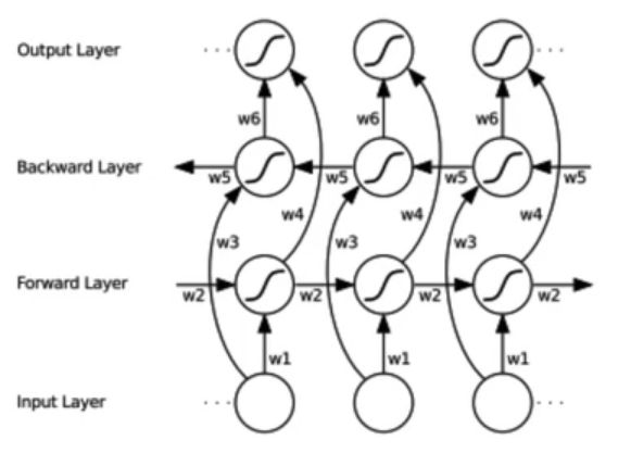
既能看到过去又能看到未来。
优缺点
优点:
- 可以处理变长序列(权重在每一时刻共享)
- 模型大小与序列长度无关
- 计算量与序列长度呈线性增长
- 考虑历史信息(隐含层)
- 便于流式输出
- 权重时不变
缺点:
1.串行计算比较慢
2.无法获取太长的历史信息 (Transformer可以)
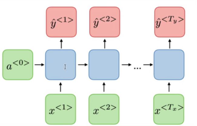
应用场景
-
AI诗歌生成(one2many)

-
文本情感分类(many2one)

-
词法识别(many2many)
-
机器翻译(many2many)seq2seq有编码器和解码器中间有attention帮助解码器

-
语音识别/合成
-
语言模型
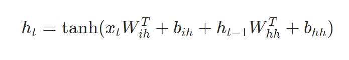
具体公式
可以看作是对输入 x t x_t xt和前一个隐含层的状态 h t − 1 h_{t-1} ht−1的一个线性层。权重加偏置,然后就是一个非线性层tanh或者ReLU。
主要参考自
https://www.bilibili.com/video/BV13i4y1R7jB/?spm_id_from=333.999.0.0&vd_source=5413f4289a5882463411525768a1ee27