多传感器时频信号处理：多通道非平稳数据的分析工具（Matlab代码实现）

欢迎来到本博客❤️❤️

博主优势：博客内容尽量做到思维缜密，逻辑清晰，为了方便读者。

⛳️座右铭：行百里者，半于九十。

本文目录如下：

目录

1 概述

2 运行结果

3 Matlab代码实现

4 参考文献

---

1 概述

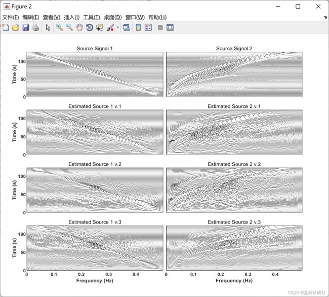
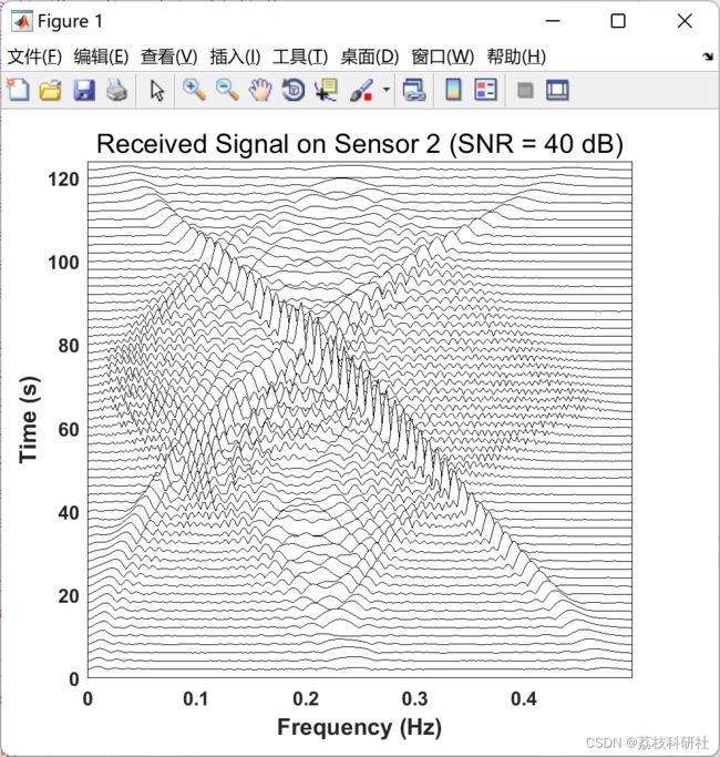
本文可塑造性强。 本文介绍了高分辨率多传感器时频分布（MTFD）及其在多通道非平稳信号分析中的应用。该方法结合了高分辨率时频分析和阵列信号处理方法。MTFD的性能通过多种应用进行了演示，包括基于到达方向（DOA）估计的源定位和非平稳源的自动组分分离（ACS），重点是盲源分离。MTFD方法通过脑电图信号的两个应用进一步说明。一种专门使用 ACS 和 DOA 估计方法进行伪影去除和源定位。另一种使用MTFD进行跨渠道因果关系分析。本文可以换上自己的数据，并将这些方法实现。

2 运行结果

 部分代码：

clear; close all; clc;
addpath(genpath('Supporting functions'));

%% Main

%% Extracting SNR information from Data Folders
S = dir('../data/DOA Data');
SNR_N = sum([S(~ismember({S.name},{'.','..'})).isdir]);
SNR_i = zeros(1,SNR_N);
for i = 1:SNR_N
    [~, r1] = strtok(S(7+i).name);
    [s1, rrr] = strtok(r1);
    SNR_i(1,i) = str2double(s1);
end
SNR_i = sort(SNR_i);
%% MUSIC and TF-MUSIC Spectrum
SNR_N = 2;
figure('Color',[1 1 1],'Position',[100, 70, 900 500]);
ha = tight_subplot(SNR_N/2,2,[0.05 0.01],[0.12 0.12],[0.08 0.08]);
for i = 1:SNR_N
    Path = ['../data/DOA Data/SNR ' num2str(SNR_i(i)), ' dB'];
    load([Path '/Averaged_Spectrum']);
    axes(ha(i));
    plot(theta, P_tf_music_avg,'-b','linewidth',2); hold on;
    plot(theta, P_music_avg,'-.r','linewidth',2); hold on;
    plot(repmat(ra(1),10),linspace(0,1.2,10),'k--','linewidth',2); hold on
    plot(repmat(ra(2),10),linspace(0,1.2,10),'k--','linewidth',2); grid on
    axis([0 39.9 0 1.2])
    if(mod(i,2) && i < SNR_N-1)
        set(gca,'XTickLabel','','fontweight','bold','fontsize',13);
        ylabel('P_M_U_S_I_C (\theta)','Fontsize',16);
        title(['SNR = ' num2str(SNR_i(i)), ' dB'],'fontsize',20);
    elseif i == SNR_N-1
        set(gca,'fontweight','bold','fontsize',13);
        ylabel('P_M_U_S_I_C (\theta)','Fontsize',16);
        xlabel('\theta (deg)','Fontsize',16);
        title(['SNR = ' num2str(SNR_i(i)), ' dB'],'fontsize',20);
    elseif i == SNR_N
        set(gca,'YTickLabel','','fontweight','bold','fontsize',13);
        xlabel('\theta (deg)','Fontsize',16);
        title(['SNR = ' num2str(SNR_i(i)), ' dB'],'fontsize',20);
        legend('TF-MUSIC Averaged Spectrum','MUSIC Averaged Spectrum','True Angles','Location','Southwest')
    else
        set(gca,'XTickLabel','','YTickLabel','','fontweight','bold');
        title(['SNR = ' num2str(SNR_i(i)), ' dB'],'fontsize',20);
    end
end
set(gcf,'Units','inches'); screenposition = get(gcf,'Position');
set(gcf,'PaperPosition',[0 0 screenposition(3:4)],'PaperSize',screenposition(3:4));

%% DOA NMSE
SNR_N = sum([S(~ismember({S.name},{'.','..'})).isdir]);
Path = ['../data/DOA Data/SNR ' num2str(SNR_i(i)), ' dB'];
load([Path '/DOA'],'ra');
nmse_music     = zeros(length(ra), SNR_N);
nmse_tf_music  = zeros(length(ra), SNR_N);
nmse_esprit    = zeros(length(ra), SNR_N);
nmse_tf_esprit = zeros(length(ra), SNR_N);
music_rate    = zeros(length(ra), SNR_N);
tf_music_rate = zeros(length(ra), SNR_N);
for i = 1:SNR_N
    Path = ['../data/DOA Data/SNR ' num2str(SNR_i(i)), ' dB'];
    load([Path '/DOA']);
    for j = 1:length(ra)
        temp1 = DOA_music(:,j); temp2 = DOA_tf_music(:,j);
        music_rate(j,i)    = sum(temp1~=0)/length(temp1);
        tf_music_rate(j,i) = sum(temp2~=0)/length(temp2);
        temp1 = temp1(temp1~=0); temp2 = temp2(temp2~=0);
        nmse_music(j,i)     = (mean(((temp1 - ra(j))/ra(j)).^2));
        nmse_tf_music(j,i)  = (mean(((temp2 - ra(j))/ra(j)).^2));
        nmse_esprit(j,i)    = (mean(((DOA_esprit(:,j) - ra(j))/ra(j)).^2));
        nmse_tf_esprit(j,i) = (mean(((DOA_tf_esprit(:,j) - ra(j))/ra(j)).^2));
    end
end
fprintf(2,'Mean Probability of Detection (Pd)\n');
fprintf('MUSIC     : %0.3f\n',mean(mean(music_rate)));
fprintf('TF_MUSIC  : %0.3f\n',mean(mean(tf_music_rate)))
fprintf('ESPRIT    : %0.1f\n',1)
fprintf('TF_ESPRIT : %0.1f\n',1)
figure('Color',[1 1 1],'Position',[100, 10, 650, 550]);
ha = tight_subplot(1,1,[0.01 0.01],[0.12 0.1],[0.12 0.12]);
axes(ha(1));
plot(SNR_i,10*log10(mean(nmse_tf_music)),'-b','linewidth',2);  hold on;
plot(SNR_i,10*log10(mean(nmse_music)),'--b','linewidth',2);    hold on;
plot(SNR_i,10*log10(mean(nmse_tf_esprit)),'-.r','linewidth',2); hold on;
plot(SNR_i,10*log10(mean(nmse_esprit)),':r','linewidth',2);   grid on;
xlim([SNR_i(1) SNR_i(end)]);
legend('TF-MUSIC','MUSIC','TF-ESPRIT','ESPRIT','Location','Southwest');
set(gca,'fontweight','bold','fontsize',14);
title('DOA Normalized Mean Square Error','fontsize',18);
xlabel('SNR (dB)'); ylabel('NMSE (dB)');
set(gcf,'Units','inches'); screenposition = get(gcf,'Position');
set(gcf,'PaperPosition',[0 0 screenposition(3:4)],'PaperSize',screenposition(3:4));

%% DOA PDFs
SNR_N = 2;
bins_N = 100;
for i = 1:SNR_N
    aa= figure('Color',[1 1 1],'Position',[100, 0, 650, 700]);
    ha = tight_subplot(2,1,[0.01 0.01],[0.1 0.1],[0.05 0.05]);
    Path = ['../data/DOA Data/SNR ' num2str(SNR_i(i)), ' dB'];
    load([Path '/DOA']);
    axes(ha(1)); temp = DOA_music; temp = temp(temp~=0);
    histogram(temp, bins_N,'Normalization','probability','facecolor',[1 0.84 0],'linewidth',1.2); hold on;
    temp = DOA_tf_music; temp = temp(temp~=0);
    histogram(temp, bins_N,'Normalization','probability',...
        'facecolor',[1 0 0],'linewidth',1.2); xlim([0 40]);
    temp1 = DOA_music(:,1); temp1 = temp1(temp1~=0); u1 = mean(temp1); s = std(temp1);
    tag11 = ['\mu_1 = ', num2str(round(u1,1)), ', \sigma_1 = ', num2str(round(s,1))];
    temp1 = DOA_music(:,2); temp1 = temp1(temp1~=0); u1 = mean(temp1); s = std(temp1);
    tag12 = ['\mu_2 = ', num2str(round(u1,1)), ', \sigma_2 = ', num2str(round(s,1))];
    tag1 = ['         MUSIC' char(10) tag11 char(10) tag12];
    temp1 = DOA_tf_music(:,1); temp1 = temp1(temp1~=0); u1 = mean(temp1); s = std(temp1);
    tag11 = ['\mu_1 = ', num2str(round(u1,1)), ', \sigma_1 = ', num2str(round(s,1))];
    temp1 = DOA_tf_music(:,2); temp1 = temp1(temp1~=0); u1 = mean(temp1); s = std(temp1);
    tag12 = ['\mu_2 = ', num2str(round(u1,1)), ', \sigma_2 = ', num2str(round(s,1))];
    tag2 = ['       TF-MUSIC' char(10) tag11 char(10) tag12];
    legend(tag1, tag2,'Location','Northwest'); grid on;
    set(gca,'XTickLabel','','YTickLabel','','fontweight','bold','fontsize',13);
    title(['SNR = ' num2str(SNR_i(i)), ' dB'],'fontsize',20);
    axes(ha(2));
    histogram(DOA_esprit, bins_N,'Normalization','probability',...
        'facecolor',[0 0.5 0],'linewidth',1.2); hold on;
    histogram(DOA_tf_esprit, bins_N,'Normalization','probability',...
        'facecolor',[0 0.45 0.74],'linewidth',1.2); xlim([0 40]);
    temp1 = DOA_esprit(:,1); u1 = mean(temp1); s = std(temp1);
    tag11 = ['\mu_1 = ', num2str(round(u1,1)), ', \sigma_1 = ', num2str(round(s,1))];
    temp1 = DOA_esprit(:,2); u1 = mean(temp1); s = std(temp1);
    tag12 = ['\mu_2 = ', num2str(round(u1,1)), ', \sigma_2 = ', num2str(round(s,1))];
    tag1 = ['         ESPRIT' char(10) tag11 char(10) tag12];
    temp1 = DOA_tf_esprit(:,1); u1 = mean(temp1); s = std(temp1);
    tag11 = ['\mu_1 = ', num2str(round(u1,1)), ', \sigma_1 = ', num2str(round(s,1))];
    temp1 = DOA_tf_esprit(:,2); u1 = mean(temp1); s = std(temp1);
    tag12 = ['\mu_2 = ', num2str(round(u1,1)), ', \sigma_2 = ', num2str(round(s,1))];
    tag2 = ['       TF-ESPRIT' char(10) tag11 char(10) tag12];
    legend(tag1, tag2,'Location','Northwest'); grid on;
    set(gca,'YTickLabel','','fontweight','bold','fontsize',13);
    xlabel('\theta (deg)');
    set(gcf,'Units','inches'); screenposition = get(gcf,'Position');
    set(gcf,'PaperPosition',[0 0 screenposition(3:4)],'PaperSize',screenposition(3:4));
end

3 Matlab代码实现

4 参考文献

部分理论来源于网络，如有侵权请联系删除。

[1] B. Boashash, A. Aissa-El-Bey, M. F. Al-Sa'd, Multisensor Time-Frequency Signal Processing:
    A tutorial review with illustrations in selected application areas, Digital Signal Processing, In Press.
[2] B. Boashash, A. Aissa-El-Bey, M. F. Al-Sa'd, Multisensor time-frequency signal processing software Matlab package: An analysis tool for multichannel non-stationary data , SoftwareX, In Press.