（八）梯度下降法

一、 梯度下降法

1.1 梯度

       本意是一个向量（矢量），表示某一函数在该点处的方向导数沿着该方向取得最大值，即函数在该点处沿着该方向变化最快，变化率最大

梯度下降：梯度下降法的计算过程就是沿梯度下降的方向求解极小值；对于一个损失函数，求在θ取某个值时J（损失）最小的一种思想；

不是一个机器学习算法；

基于搜索的最优化方法；

作用：最小化一个损失函数

1.2 示例

import  numpy as  np
import  matplotlib.pyplot  as plt

plot_x = np.linspace(-1, 6, 140)
plot_y = (plot_x-2.5)**2-1

# 损失函数
plt.plot(plot_x, plot_y)
plt.show()

1.3 原理  

       J最小时该函数θ处导数为0；梯度下降时每一次取到的J都应比上一次小

plot_x = np.linspace(-1, 6, 200)
plot_y = (plot_x-2.5)**2-1

# ------计算θ处的倒数
def dJ(theta):
    return 2*(theta-2.5)

# ------θ处J的值
def J(theta):
    try :
        return (theta-2.5)**2 - 1.
    except:
        return float('inf')


# ------梯度下降
# init_theta：初始θ值
# eta：学习率，也就是步长
# n_iters：收敛速度和eta值相关，eta太小收敛慢
# epsilon：要求精度
def gradient_descent(init_theta, eta, n_iters=10000, epsilon=1e-8):
    theta = init_theta
    theta_history.append(init_theta)
    i_iters = 0
    
    while i_iters < n_iters:
        gradient = dJ(theta)  
        last_theta = theta

        # 下一个θ值
        theta = theta - eta * gradient
        # 把所有取过的θ放到theta_history中，为画图做准备
        theta_history.append(theta)
        # 当两次差值小于要求精度epsilon时，跳出函数，此时找到了θ
        if(abs(J(theta)-J(last_theta)) < epsilon):
            break
        # 循环次数累积
        i_iters+= 1

# ------绘制下降曲线       
def plot_theta_history():
    plt.plot(plot_x, J(plot_x))
    plt.plot(np.array(theta_history), J(np.array(theta_history)),color = 'r', marker='+')
    plt.show()

1.4 不同eta对梯度下降结果的影响

① eta取0.01：学习率太小，收敛时间太长

eta = 0.01  
theta_history = []
gradient_descent(0.,eta)
plot_theta_history()
len(theta_history)

② eta取0.1

eta = 0.1  
theta_history = []
gradient_descent(0.,eta)
plot_theta_history()
len(theta_history)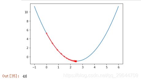

 

③ eta取0.8

eta = 0.8 
theta_history = []
gradient_descent(0.,eta)
plot_theta_history()
len(theta_history)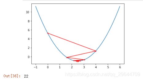

 

④ eta取1.1：学习率太大，离预期越来越远，最后抛出异常

eta = 1.1
theta_history = []
gradient_descent(0.,eta,n_iters=10)
plot_theta_history()
len(theta_history)

 

theta_history
'''
[0.0,
 5.5,
 -1.1000000000000005,
 6.820000000000001,
 -2.684000000000002,
 8.720800000000004,
 -4.964960000000007,
 11.457952000000008,
 -8.249542400000012,
 15.399450880000016,
 -12.979341056000022]
'''

二、随机梯度下降法

批量梯度下降：对所有样本进行计算，搜索沿着损失函数减小最快的方向逐渐下降，当样本量很大时收敛速度会很慢；

随机梯度下降，只选出一个样本进行计算，不能保证搜索方向一定是损失函数减小的方向，也不能保证是减小最快的方向，但最后一定会找到或者靠近最小的损失函数，用少量的数据样本计算，大大缩短了收敛时间；

随机梯度下降法：很有可能跳出局部最优解，找到全局最优解。

import numpy as np
import matplotlib.pylab as plt
from sklearn import datasets

boston = datasets.load_boston()
x = boston.data
y = boston.target

# 数据清洗
X = x[y<50]
y = y[y<50]

from  sklearn.model_selection  import  train_test_split

X_train, X_test, y_train, y_test = train_test_split(X,y,test_size=0.2,random_state=666)

# 数据归一化
from  sklearn.preprocessing  import  StandardScaler

scaler = StandardScaler()
scaler.fit(X_train)
X_train_scaler = scaler.transform(X_train)
X_test_scaler = scaler.transform(X_test)

from sklearn.linear_model  import SGDRegressor

sgd = SGDRegressor()
sgd.fit(X_train_scaler,y_train)
sgd.score(X_test_scaler,y_test)

#  0.8129534790265714